10.1 Objectives

In this lab you will:

1. Create a geodatabase to contain existing data for the field area we will visit this weekend;
2. Create a feature dataset containing empty polygon, line and point feature classes with domains for field data entry;
3. Create a project containing all data needed for field data collection;
4. Print layouts and instructions for data collection to take with you to the field;
5. Export your project to an ArcPad project;
6. Review procedures for capturing GPS points, lines and polygons with ArcPad software;

10.2 Geodatabase Preparation with ArcGIS 9.2

Most data for this project are available in shapefile format, but we will find it useful to build a geodatabase so that we can establish domains for data entry.  We will be collecting data with ArcPad software, which permits the capture of GPS positions for points and vertices and uses forms for entering attributes while in the field.  By using coded value domains in our geodatabase, we can create drop-down menus for our forms, a far easier way to enter attributes than pecking letters with a stylus on a virtual keyboard.  Recent versions of ArcGIS (9.0 and above) also allow the option of "checking out" Feature Classes from a database for field editing with ArcPad, then checking them back in when finished.  When it works properly, this is a very efficient way of creating a field-based GIS, eliminating the need to update existing files by appending, merging or otherwise editing them to conform to new field data.  You have already done many of the steps below in Lab 5. Refer to it if you've forgotten aspects of geodatabase Feature Class and Domain creation.

1. Download the Lab_10_data folder to your personal storage space.
    
2. Open ArcCatalog and browse to your Lab_10_data folder.
    
3. Create a personal geodatabase called "Mason_Mt_WMA" (= Wildlife Management Area) within the Lab_10_data folder.
    
4. Right-click on your new geodatabase and import all of the Feature Classes in the Lab_10_data folder (and subfolders) into the geodatabase. The spatial reference for all of these feature classes is NAD83, UTM zone 14N, and they will import as such.
    
5. Geodatabases can not hold layer files (these files contain the symbology for the feature classes you just imported) yet we would like to use the layer files to symbolize the new geodatabase feature classes. To do so we must reset the source for the layer files.
   
   Right-click on a layer file icon, select "Properties...", click the Source tab then the "Set Data Source..." button and reset the source by browsing to the appropriate Feature Class in your geodatabase. Do this for all Feature Class layer files (but not raster layer files).
    
6. What about the raster files?  The lab_10_data folder contains a DOQ and hillshade raster with associated layer files; should we import these into the geodatabase? In this case the disadvantages of doing so outweigh any advantage. In particular, the color DOQ is a large MrSID file that would get much larger when uncompressed and stored in IMG format, which is the format required by the geodatabase. There is no real advantage to doing this, other than having everything in a single container, and we are left with a file that is >150 Mb instead of <20 Mb, a much more manageable file size. We could instead create a geodatabase raster index (see Help files on this topic), but for the few rasters we will work with this also provides no real advantage. We will keep the rasters separate from the geodatabase for these reasons.
    
7. Time to create the empty Feature Classes that will contain the GPS-derived points lines and areas... 

1. Before doing so, it is good practice to create a Feature Dataset that will contain the Feature Classes.  To do so, right-click on the Mason_Mt_WMA geodatabase icon, select "New...", then create a new Feature Dataset called "Geology".  SET THE SPATIAL REFERENCE OF THE FEATURE DATASET TO NAD83 UTM zone 14N, SET THE "Z COORDINATE SYSTEM" TO <None>
   AND ACCEPT THE DEFAULT XY TOLERANCES. (Note for outside users: the procedure for doing this in ArcGIS 9.1 is somewhat different.  See an example here)
   
2. Now we can create the Feature Classes; right-click on the Geology Feature Dataset icon, select "New...", then create new Polygon, Line and Point Feature Classes (named Polygon, Line and Point).  Do this step 3 times, one for each Feature Class, being sure to change the Geometry type [polygon, line, point] to match the Feature Class and checking on the Geometry Properties  "Coordinates include Z Values" box.
    
3. The polygon feature class will be used to store the GPS-derived outline of granite outcrops and any other features that are polygons.  We need an attribute field that records the feature being mapped (e.g. "granite", "pegmatite" or “other”) that can be entered as we collect the data.  So... add two Text fields to the polygon feature class, one called FEATURE and another called COMMENT. The length of the FEATURE field should be 9 and the COMMENT field 30.  Leave all other Field Properties blank for now.
    
4. Create a Domain (by right-clicking on the Mason_Mt_WMA geodatabase icon, then Properties...) called PLY_TYPE, (Field Type is Text) that is a coded-value domain containing the coded values of "granite", "pegmatite", and "other" (see Lab 5) and then attach this domain to the polygon attribute field FEATURE (again see Lab 5).
   
   
5. The line Feature Class will be used to store rock unit contacts or outcrop boundaries that can't immediately be seen to close on themselves (i.e. can’t be mapped as polygons). The attributes that will be recorded and the new fields to create are:
   
   1. 9-character text field that will contain coded values from a text Domain called "LN_TYPE" of "contact", "outcrop" and "other".
   
   2. 7-character text field that will contain coded values from a text Domain called "Symbol" of "solid", "dashed" and "dotted".
   
   3. 30 character text field without an attached domain.
   
   
6. Create these new Fields and their Domains with the above coded values and attach the Domains to the Fields, as in steps c and f.
   
   
7. The point Feature Class will be used to record the location of features too small to recorded as polygons and for strike and dip measurements. We will need fields for:
   
   1. 10-character text field that will contain coded values from a text Domain called "PT_TYPE" of "foliation", "bedding", "joint" and "other".
   
   2. 3-character short integer field (Precision equals 3) that will contain coded values from a short integer Domain called "strike" of every third integers between 0 and 357 (i.e. Codes of 0, 3, 6, 9, 12 etc. with Descriptions of 000, 003, 006, 009, 012, etc. to 357; yes, all 120 values).
   
   3. 2-character short integer field (Precision equals 2) that will contain coded values from a short integer Domain called “dip” of every second integer between 2 and 90 (i.e. Codes of 2, 4, 6, etc., with Descriptions of 02, 04, 06 etc.; 44 values in all).
   
   4. 30-character text field, "COMMENT", without an attached domain.
   
   
8. Create these new Fields and their Domains with the above coded values and attach the Domains to the Fields, as in steps c and d.

Congratulations, you have now completed the database you will need for this project.

10.3 Making Field Maps

1. Open ArcMap with an empty map document and load all of the LAYER FILES (not the Feature Classes), including the layer files for the DOQ and Hillshade.  If this doesn't work, you skipped step 5 above.
   
   
2. Load the empty polygon, line and point Feature Classes you just created and move them to the top of the Table of Contents if not already there.
   
   
3. Order the remaining layers so that the Hillshade is at the bottom, the DOQ is second from the bottom, and all remaining layers above these.
   
   
4. Zoom to the WMA boundary layer, reset the reference scale, and SAVE THE MAP document to your Lab 10 folder.

Switch to Layout mode and make a map with a 50 meter UTM grid, scale bar, north arrow, name, etc.  Print two maps, one with the hillshade layer turned on and another with the hillshade off but the DOQ on. The scale should be ~ 1:10,000 to be useful; you will have to tile the map onto a few pieces of paper to cover the area of interest (Ephraim will tell you how much of the area to print), which is within the portion of the WMA that is south of Mason Mountain.  Bring these maps with you on the field trip.

10.4 For Trimble GeoXT and Xplore Tablet Users

GPS data collection using the Trimble GeoXT, the In-Situ Rugged Reader Field Units/TDS Recon, and Xplore Tablets is best done with ArcPad software.  ArcPad is a streamlined version of ArcGIS that is equipped with very easy to use GPS capture tools.  ArcPad 7.x is installed on the classroom computers.  Before getting a little ArcPad practice, we first need to convert the ArcGIS map document file into an ArcPad project.  An automated tool exists to do so, which converts most rasters to MrSid images, the geodatabase feature classes to shapefiles, and makes data entry forms from the domains for each Feature Class.  We can "check out" the empty Feature Classes for editing then, upon return, "check in" the same, permitting the software to automatically update the geodatabase!

An important note about ArcPad versions:

• ArcPad 7.x represents a significant departure from earlier versions (i.e. 6.x and below).  Projects created for ArcPad 7.x will not run on 6.x software, and vice-versa.  The ArcMap toolbar for creating ArcPad projects in versions of ArcGIS 9.1 and higher contains separate tools for creating ArcPad 7.x and 6.x (or lower) projects.  It is thus important to know which version of ArcPad is installed on your field data collection units.  Our Xplore tablet PCs are running ArcPad 7.x, as are the computers in the lab and the In-Situ units, but our Trimble GeoXT is still running 6.x.  If you plan on using the GeoXT, create an ArcPad 6.x project in addition to an ArcPad 7.x project.

A. Preparing the Map Document for ArcPad (version 7.x).

1. Open your map document.
    
2. Switch to Data View mode (if you're in Layout mode) and zoom to the WMA_boundary layer.  This is an important step!
    
3. Make sure the "Points", "Lines" and "Polygon" Feature Classes are present in the table of contents of the map.  These are empty, but have coded-value domains already built that will allow use of ArcPad data entry forms.  These are the files you will populate with GPS measurements.
    
4. Change the symbology of these files to colors/symbols that will be recognizable on both a white background and the DOQ.  Red works well, as does light blue.  This is much easier to do now than later in ArcPad.
    
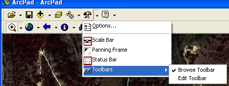
5. If not already on. Turn on the ArcPad toolbar (Tools>customize...) shown below.
    

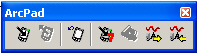
6. On the ArcPad toolbar, click the "Get Data for ArcPad 7" button .
    
7. In the "Choose layers you want to get from map" window, select everything but the raster layers (i.e. leave unchecked the Hillshade and DOQ).  The DOQ is too large to make a Mr.SID raster using the ArcPad export tool. The Hillshade will be of little use in the field and would require a lot of storage space (important for the GeoXT, but not for the tablets).  A DOQ MrSID file has been generated for you and is available in the Lab7_data folder.  Click Next.
    
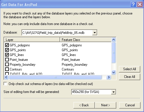
8. You now get to choose which layers you want to check out from the geodatabase.  The only ones you will edit in the field are the Points, Polygons and Lines feature classes.  Place a check next to these and leave the others blank.
    
9. DO NOT CLICK OK YET.  If you will be using a Tablet computer set the "Size of Editing form..." drop-down menu to one of the larger size, e.g. 450x290, as in the example below.  If you will be using the GeoXT or an In-Situ field unit, set the editing form size to 130x130.

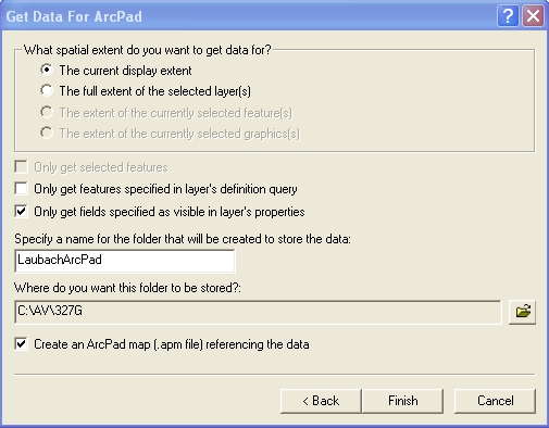
10. The final window lets you set the spatial extent (current display extent or full extent of the layers), lets you select whether to limit the fields to those that are visible in the attribute tables and the features to those specified in the layer's definition query, lets you specify a name for the folder that will store the data, and lets you create an ArcPad map file (the equivalent of an .mxd file) for the data, as shown in the "Get Data For ArcPad" screen capture below.
     
11. Enter a name for the folder, e.g. "ArcPad_WMA"
     
12. Making sure first that your display shows the entire area of interest (i.e. you are zoomed to the WMA boundary layer), make the selections shown in the figure below, setting the "Where do you want the folder to be stored?" to an appropriate location on your network storage space.

13. Click Finish and wait for the data to be created.
     
14. Within ArcCatalog, copy the DOQ.sid file from your Lab07_data folder to the new "ArcPad_WMA" folder. 
     
15. With help from Dr. H. or Ephraim, transfer your new "ArcPad_WMA" folder to the GeoXT, an In-Situ unit, or a tablet computer.  The In-Situ units have a folder called "327G" that should be used for all ArcPad data and files.

7.5 Using ArcPad - some practice with the basics

Editing in ArcPad is, in most ways, much simpler than Editing in ArcGIS.  Below are a few of the basics.  A complete description of the software can be found in the ArcPad 7 folder in the class folder or here.  A very useful Quick Reference "cheat sheet" is there as well (and here) - print one in color and take it to the field with you.

1. On a classroom computer, open ArcPad 7 from the Start Button>All Programs menu in Windows.
    
2. Click the folder button at the top of the ArcPad window and select  "Open Map", then browse to the "ArcPad.apm" file in the "ArcPad_WMA" folder.  This should load all but the DOQ.
    
3. Add the DOQ MrSID by clicking the plus button and browsing to it.  To browse, click the folder button in the "Add Layers" window, find the ArcPad_WMA folder, click OK, then check on the layer you want and click OK.
    
4. Once all the layers are loaded, Save the map.  This will ensure that next time you open this ArcPad map, you won't have to re-add the photos.
    
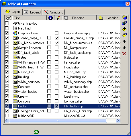
5. Click the Layers icon to open up a Table of Contents, like that shown below.

5. The check boxes on the left in the "eye" column turn layers on and off for viewing.  The check boxes in the "pencil" column turn layers on and off for editing.  This is similar to setting the "Target" of the editing toolbar in ArcGIS, except that in ArcPad more than one layer can be open for editing at a time.  In the Table of Contents above 3 layers are open for editing: a point (DK_Measurements), a polygon (Granite_outcrops_06) and a line (Faults) layer are open for editing.  Finally, the check boxes below the Info icon make layers available for query.

6. Turn on the "GPS_points" layer for editing and close the Layers window.

7. Turn on the Edit toolbar by selecting it from beneath the down arrow key, shown below.

8. The function of the edit tools are shown in the figure (from ESRI) below.

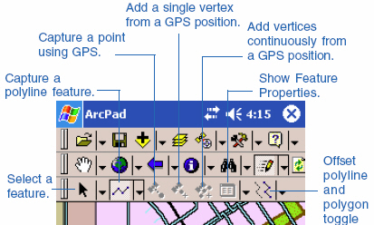
To add a point to the map, click the "Capture a point feature" button, located by clicking the black triangle to the right of the "Capture a polyline feature", then selecting the point feature from the drop-down menu. Then click a location on the map.  A data entry form should then open, allowing you to select the feature name from a drop down list.

To add a GPS location as a point, instead click the "Capture a point using GPS" button. (When the GPS is active this button is not grayed-out.)

9. To add a line, click the Layer icon, check-mark the GPS_line layer for editing, close the Layers window, click the drop-down arrow next to the "Capture a point feature" button, and select "Polyline".  Click on the map where you wish to place a polyline vertex, click and drag on the next spot where you want a vertex, and continue this process until finished.  The line is not completed until you click the "Proceed or complete feature" button at the bottom of the ArcPad window (shown below).

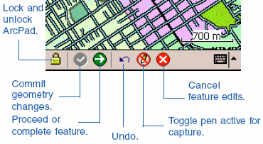
10. To add GPS vertices to a polyline, as above, click the "Capture a polyline" button (beneath the capture a point button), click the "Add a single vertex from a GPS position" button and continue clicking this button every time you want to add a vertex to the line.  To finish the line, click the "Proceed or complete feature" button. The line is not completed until you click the "Proceed or complete feature" button.
    
    The GPS must be activated before the GPS buttons are available.  We'll go over that aspect in the field.
     

11. A similar procedure is used to capture polygon vertices with and without GPS.

12. You can delete features by selecting them with the Arrow button (shown above) and then clicking the "Edit vertices" button.

13. Practice adding and deleting lines, points and polygons to the map.  Name the features test1, test2, etc. so that, if needed, you will be able to recognize and delete them later.

14. Browse the ArcPad manual in the digital books folder, particularly the sections on editing.  Download and print the ArcPad Quick Reference page.

15. If you would like practice using ArcPad with a GPS, an ArcPad project for the East Mall, identical to the ArcGIS project you constructed in Lab 9, is loaded on all instruments.  Take your instrument outside, load the East Mall project, and practice capturing lines and points.

Before loading your WMA ArcPad folders to the field GPS units, clear each of your test features.

That's all for now, with more to come on completing a map with the data you collect.