Introduction

In this lab, you will manipulate several vector and raster data sets using the Spatial Analyst extension and ArcToolbox Tools to produce four raster layers to analyze for erosion susceptibility in Yellowstone National Park.

The Problem

Where will problems with surface runoff and erosion be greatest in Yellowstone National Park after the fires of 1988?

Goal

To solve our problem, we will create a “suitability” map of Yellowstone National Park showing ranking (from 3 to 16) of potential for runoff and erosion problems at a resolution of 100 m².

A. Breakdown of the Problem

1. What are the objectives needed to reach the goal ?

a. Identify key factors that affect runoff and erosion:

• Slope
• Rock type
• Recent (since 1988) loss of vegetation to fires
• Precipitation

b. What is the relative importance of these factors? i.e. How will each be ranked and weighted?

We will use a scale of 0-4 for each factor, with 4 being the most important. The table below specifies which values correspond to which rank for each of the four factors. Note that a rank of zero is only used for the burn factor, and it is only applied to unburned areas. All other factors will have a value between 1 and 4.

Basically, each raster cell in the study area will receive an ordinal rank for each of the four factors. Each cell’s ranks will be totaled in order to determine its suitability. For example, a raster cell whose geology is tuff (rank = 3), has a slope of 4^o(rank = 1), is burned (rank = 4), and receives 50 inches of precipitation per year (rank = 3) will have a total “suitability” score of 11 (3 + 1 + 4 + 3 = 11). Suitability scores will range from 3 to 16. The higher the score, the more susceptible the area occupied by the raster is to erosion.

2. What data sets are needed?

We know that to apply our ranking scheme to achieve our goals, we need a GIS layer for rock type, slope, burn cover, and annual precipitation. In some cases, we may find the needed data ready to use and will only have to reclassify it to match our ranking scheme. In others, we will need to convert vector data to grids and/or derive the needed data from the primary data before reclassifying. Our data needs are summarized below:

B. Explore the Primary Data Sets

• Copy the Lab_11_data folder to your network storage space.
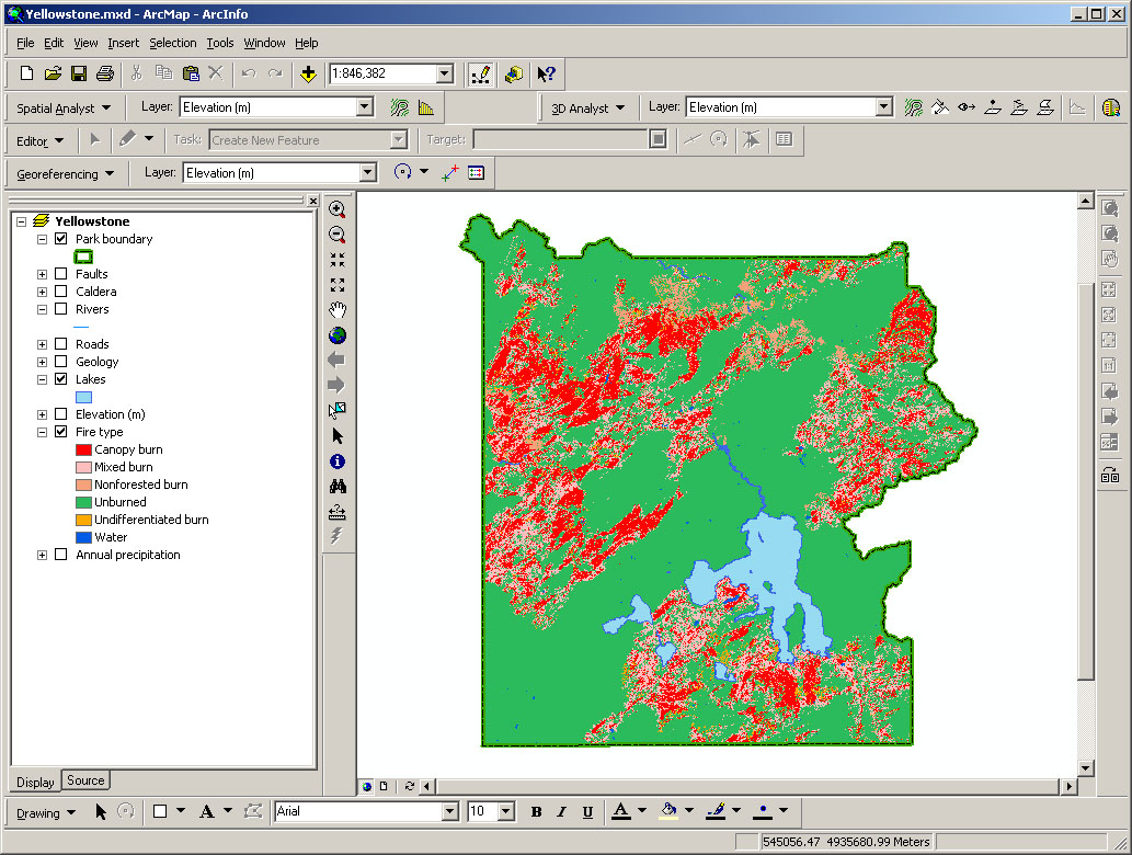
• Open the ArcMap file Yellowstone.mxd. You should see a map of Yellowstone Park showing the park boundary, areas affected by fires (since 1988), rivers, and lakes. Several other layers are included, though they are currently not displayed. Explore the various data sets, and answer the questions below.

1. Rasters:

The resolution and extent of each raster layer must be known. In order to perform spatial analyses, all rasters should share a common resolution and the same spatial extent must be used.

C. Perform Analysis

1. Preprocessing of primary data sets:

a. Projection: Set GCS, PCS, create .prj files; project files as needed. (THIS HAS ALREADY BEEN DONE FOR YOU.)

b. Set up a working directory for your spatial analyses.

• First, create a folder within the Lab11_data folder to use as your home workspace (name it something like New_Grids).
•  We will find it useful to establish several environment variables, including a mask for setting the analysis area when generating new rasters.  This can be done by selecting the Geoprocessing drop-down from the main ArcMap menu, then choosing Environments>Raster Analysis>Mask.  Set the mask to the Park_boundary polygon.  Doing so enables all new rasters to be restricted to the park boundary automatically - you will not need to set the mask for each raster operation!
• When using the Spatial Analysis tools in ArcToolbox, use the "Environments" button to set a mask using parkbnd.shp.

c. Table joins, symbolize, create layer (.lyr) files.

• The Geology attribute table has a field called PTYPE-GEN that contains abbreviations for the rock units but does not have a field that holds rock unit names for each of the abbreviations.  To create such a table, you need to join the Geology table to a .dbf table called "Geol83.lup" (a "lookup table") that is in the ofr99174\coverage folder.
• Add the Geol83.lup file to the project
• Right-click on the Geology layer in the Table of Contents and select "Joins and Relates>Join..."
• Fill in the window: The field in the geology layer and the Geol83.lup lookup that the join will be based on is the PTYPE-GEN field - it has the same name in both tables.
• After pressing OK, you may be asked if you want to create an Index for the table.  Answer Yes, though for a table this small this is not really necessary.
• A Layer file, named "Upper Cenozoic Geologic Units.lyr", can be used to symbolize the geology on the basis of the geo83.lup:Group field.

Question 4: In the chart below, indicate which attribute of each vector layer will eventually be used for ranking: Vector Layer Attribute to be used for ranking Geology   Annual precipitation

d. Aggregate and/or clip vector data.

• Although clipping to the park polygon is optional because we will eventually convert the vector data to rasters and analyze the rasters using the analysis mask, go ahead and clip the vector layers to the park boundary using the tool to do so in ArcToolbox. This will ensure your results in each subsequent step match those expected from the lab procedure.

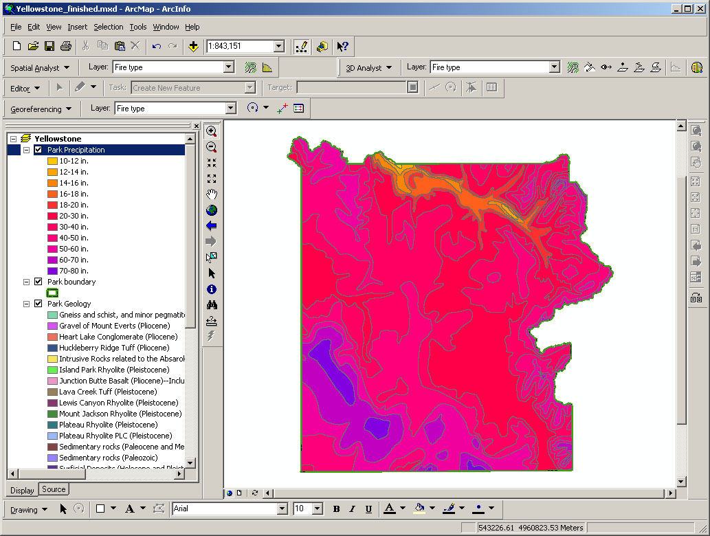
• Symbolize the clipped geology layer using "Upper Cenozoic Geologic Units.lyr" file, using the GROUP field as the "value field".

Symbolized Geology layer using the "Upper Cenozoic Geologic Units.lyr" file

• After symbolizing the clipped geology layer, aggregate all the polygons for each of the 17 values displayed for the clipped geology layer in the Table of Contents. To do this, use the Dissolve tool in the Data Management Tools>Generalization Toolbox, specifying GROUP as the "Dissolve_Field".
• Join the geol83.lup table to the now clipped and dissolved geology layer using the "geol83_l_3" as the joining fields (after clipping this field replaced geol83_l_3).
• Symbolize the output layer the same way you did for the clipped geology layer. Although the two layers look basically the same, there are only 18 records in the dissolved layer compared with over 80 records in the original clipped layer. Basically you have made one record for each geol83_l_3 value—all polygons sharing a common value have been combined into one feature and are represented by a single record in the attribute table.

-Clipped precipitation layer-

2. Derive secondary data sets from primary data sets:

a. Create slope grid.

• To create the slope grid, first display only the elevation layer and the park boundary as shown below. Note how the elevation data extends beyond the irregular park boundary. We cannot clip raster data to irregular boundaries as we can vectors, but the analysis mask discussed earlier will allow us to perform analyses only on the grid cells that are within the park boundary. The analysis mask will be applied to all subsequent raster analyses unless we forget to apply it with the "Environments" button for the tools we will use.

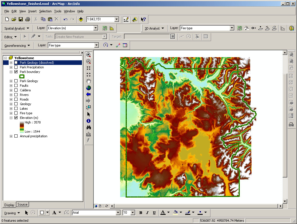
-Elevation and park boundary-

• Go to Spatial Analyst > Surface Analysis > Slope. Select Elevation (m) as the input surface, and ensure that the Output measurement is Degree, the Z factor is 1 (i.e. horizontal and vertical units are the same, in this case meters), and the Output cell size is 100. Specify an output raster, and click OK. If the slope tool fails, clear the mask in the Environments setting, use the Clip tool to clip the elevation data to the Park Boundary, then try the slope tool on this clipped version.

***Potential Bug: ArcMap may reject your slope calculation. If this happens, try again and save the output raster to the same folder that contains the ArcMap file in which the calculation is taking place, or work from your flash drive.  See also the note above about clearing the Mask in the Environments window.***

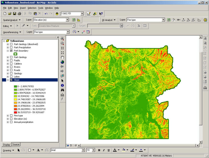
-Slope (derived from elevation) and park boundary-

b. Create geology grid from the dissolved geology vector layer, and convert the clipped precipitation vector layer to a grid.

• We must convert the geology to a raster layer in order to use it in our spatial analysis. Search ArcToolbox for the Features to Raster tool. Select the dissolved geology layer as the input, geol83_l_3 as the field, 100 as the output cell size, and an output raster name of your choice. Click OK. The conversion may take a few minutes. You should end up with a raster that looks very similar to your input vector layer.  This can not be symbolized with a vector layer file; this is now a raster and would need a raster layer file to symbolize the units.  We don't have one; leave it unsymbolized and accept the default colors.
• Repeat the process for the clipped precipitation vector layer, using CATEGORY as the field, 100 as the output cell size and specifying a new output file name. Don't forget to set the mask.  Symbolize as you did for the vector file, but this time use the Partial Spectrum Color Scheme.

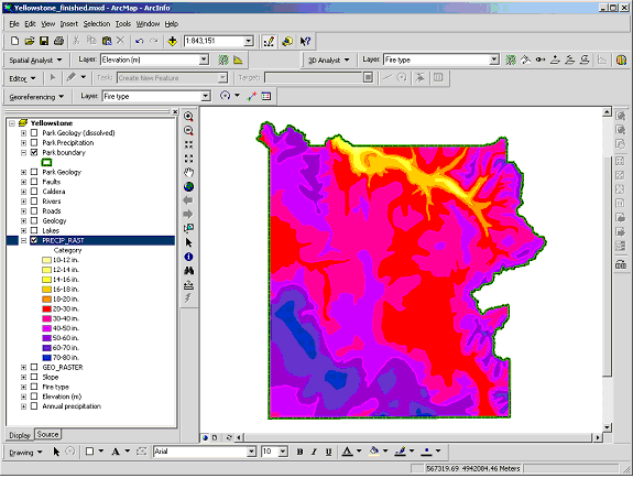
-Precipitation raster with Partial Spectrum Color Scheme-

3. Reclassify data sets:

• To reclassify the raster data sets using our ranking scale, go to Spatial Analyst > Reclassify, and input the parameters for each of the four rasters as shown below. Note that for layers with numeric data (not text), you can edit the old values as well as the new values in the Reclassify window (e.g., for slope).

***Potential Bug: ArcMap may reject your reclassification. If this happens, try again and save the output raster to the same folder that contains the ArcMap file in which the reclassification is taking place, or work from a flash drive.***

***Potential Bug: Reclassifications with several value changes may be rejected by ArcMap. If this happens, try scrolling back up through the list in the reclassify window, click values as you go along. Then pull the vertical scroll bar all the way down then up to clear any cell lines in the list. Then click OK. If this doesn’t work, consider adding a new field for rank to the vector input file, manually inputting the rank values in the new field, then reconverting the vector file to a grid using this new field.***

-Slope reclassification parameters-

• For precipitation reclassification, use Category as the Reclass field, do not edit the old values, and input the new values according to the chart at the beginning of lab.
• For fire type reclassification, water and unburned get a new value of zero, whereas all other values (except “no data”) get a new value of 4.
• For the slope reclassification, first redefine the slope interval in Symbology tab of layer Properties to a Defined Interval of 10 degrees before reclassifying using the parameters shown in the figure above.
• For geology reclassification (using the Value field in the attribute table), use the chart in the MS Word document "geology reclassificaton.docx" in the Lab 11_data folder as a guide. Note also the following specific rankings that may not be immediately apparent:
• Unattributed areas are water and should be reclassified as "NoData"
• Reclassification will not work if you use the "Name" field, even if this is presented as an option.  You must reclassify numeric values to numeric values.  Use the Value field as the "old value".  If you keep your attribute table open you can see both the value and the geological unit as you reclassify.

Again, see "geology reclassificaton.docx" for specifics.

4. Weight and combine data sets:

• We will treat each of the four factors equally, so no weighting will be used. To combine the ranked data sets and produce a composite ranking layer, go to Spatial Analyst > Raster Calculator. Double-click on one of the ranked grids listed in the upper left column, click the plus sign, double-click on a second ranked grid, click the plus sign, double-click on a third ranked grid, click the plus sign, double-click on the fourth and final ranked grid, and click Evaluate.
• Symbolize your resulting raster output using the Red to Green color scheme with the colors flipped (right-click in the symbology window and choose Flip Colors). Your final raster layer should look like the screen capture below:

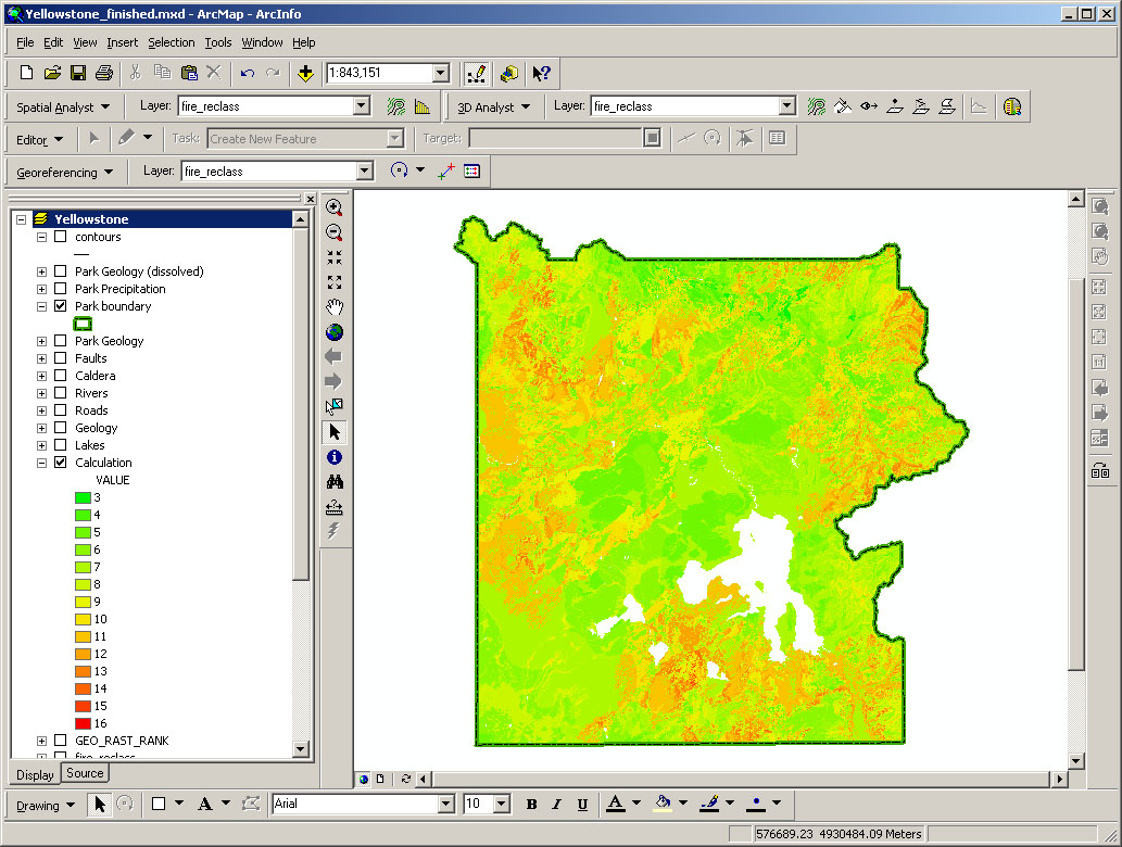
-Final output grid with erosion susceptibility ranked from 3 to 16-

Ancillary Exercises to Help You With Term Projects (yes, you have to do these exercises)

T. Pierce and M. Helper, Fall 2003, 2007, updated Fall 2014