Note Added on 10/22/14 - See these Revisions

9.1 Objectives

This Lab contains 2 parts. In Part A, to be done in lab, you will:

1. Create a Digital Elevation Model from LiDAR LAS files
2. Modify an existing Geodatabase and map to include historical river channel outlines
3. Print layouts and instructions for data collection to take with you to the field;
4. Export your project to an ArcPad v.10 project;

In Part B, to be done during the following lecture period, you will:

1. Learn procedures for capturing GPS points, lines and polygons with ArcPad 10 software;
2. In pairs, practice with a Trimble Nomad GPS receiver capturing the locations of polygons and lines on the Campus Main Building Mall.

9.2 The Problem and the Data

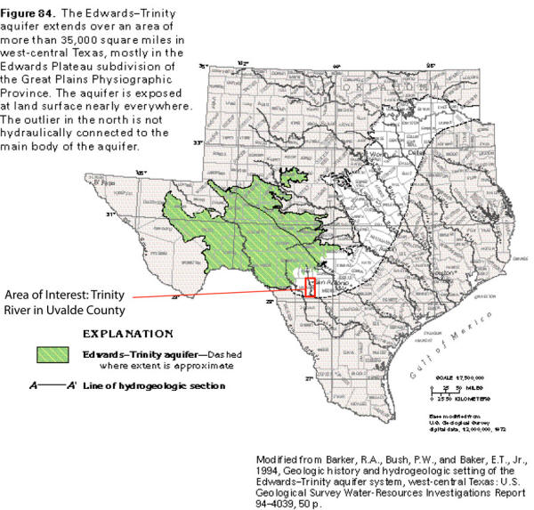
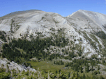
The Nueces River in Uvalde County, TX is incised into and has its headwaters on the Edwards Plateau, a large, broad expanse of Cretaceous limestone that extends from Austin south and west to near Van Horn, TX (see below).  Groundwater beneath the Plateau in our area of study is contained within the Edwards-Trinity aquifer. 

(Modified from http://pubs.usgs.gov/ha/ha730/ch_e/E-edwards_trin1.html)

Groundwater models that make predictions about aquifer characteristics rely in part on knowing how and where an aquifer receives surface water ("recharge", "recharge zone") and how water is lost ("discharged"; e.g. springs, withdrawal by wells).  Recent gauging studies of the Nueces River show it to be a potential site of recharge for the Edwards-Trinity aquifer, as indicated by flow rates and volumes that are variable along short reaches of the river.  Near our field site, downstream gauging sites show less flow than those upstream - the river is losing water into the subsurface between sites.  Two end-member hypotheses might explain this loss:

1. Nueces River water is traveling downward into the Edwards-Trinity aquifer through fractures in limestones in the river bed;

2. Water is being lost into the shallow subsurface (but not the Edwards-Trinity aquifer) via travel through relatively thick and highly permeable Nueces River fluvial deposits (gravel and sand) and flowing in buried river channels that bypass surface gauging stations.

We will evaluate these hypotheses by:

1. constructing a very high resolution elevation model of the river and its surrounding that will aid  in
2. constructing a geologic map of older, younger and modern river deposits, and of the present and relatively recent river channels;
3. noting the density and measuring the orientation of any bedrock fractures in the river bed.

Data 

For the GIS lab portion of the project we will work with the following data:

• UTM zone 14 NAD83, LAS-format Airborne LiDAR files acquired during flights in January, 2014, provided by Marcus Gary at the Edwards Aquifer Authority.
• UTM zone 14 NAD83, LiDAR intensity "maps" (panchromatic raster images) with a resolution of 0.5 m, clipped to the area of interest;
• UTM zone 14 NAD83, 1 meter-resolution digital orthophotos acquired in March,1996 and June, 2012, clipped to the area of interest, from TNRIS and Google Earth;
• UTM zone 14 NAD83 1:24,000 Digital raster graphs, clipped to the area of interest, from TNRIS;
• NAD83 edited National Hydrological Dataset (http://nhd.usgs.gov) ) files for water bodies, springs and flow lines;
• A geodatabase that contains some of the files above, as well as a feature dataset of vector files for a preliminary geologic map that I completed last week.

**Download the Lab_7_data folder to your flash drive, NOT YOUR NETWORK STORAGE.**  This file contains 2.43 Gb of data and may take up to 5 minutes to download.
 

9.3 Working with LiDAR data in ArcGIS 

LiDAR data are fundamentally clouds of points ("point clouds") with XYZ coordinates and attributes. They are commonly distributed in LAS (LASer) format files, a non-propriety format that has gained wide acceptance in recent years.  ArcGIS have extensive tools for importing and working with LAS files.  Our goals for this part of the lab are to:

• Import LAS files into ArcGIS and examine their properties
• Create a raster digital terrain model ("DTM") from these vector files

1. After checking to be sure that the Spatial Analyst and 3D Analyst Extensions are checked on in a blank ArcMap document, open the ArcCatalog window inside of ArcMap, right-click on the Lab_7_data "LiDAR" folder and select "New", create a "LAS Dataset" and rename it Nueces.lasd.  This creates a container into which we can import LAS files.  A "LAS Dataset" (.lasd) has special properties that allow us to examine some of the unique features of LiDAR data and is required for some LAS processing tools.
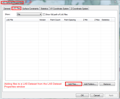
2. Add the four LAS files (each is a tile of a single large area and has a file name that ends with .las) to this new LAS Dataset by right-clicking on the LAS Dataset icon, selecting "Properties...", the "LAS Files" tab and the "Add Files..." button (shown below).

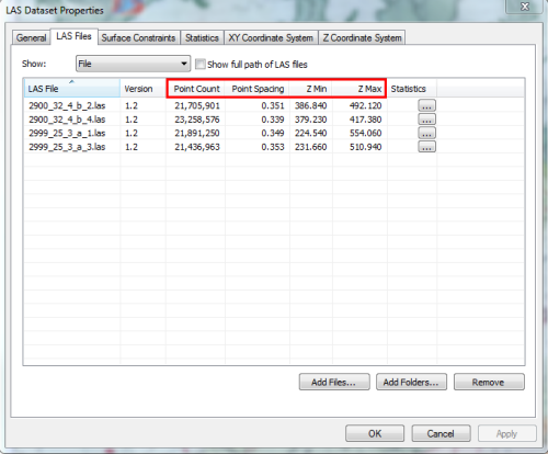
3. Examine the Properties of the imported files. Note that each file contains 21-23 million points - we will be working with over 88 million points in this exercise (!) - that are spaced at about 0.35 meters (as shown below).  The maximum (Z Max) and minimum (Z min) elevation of the points in each file is also listed.

4. Open the "Statistics" tab and click the "Calculate" button - this may take some time...
5. As shown below, the result provides Statistics on two important parameters.  This will be important later - pay attention as you read on...

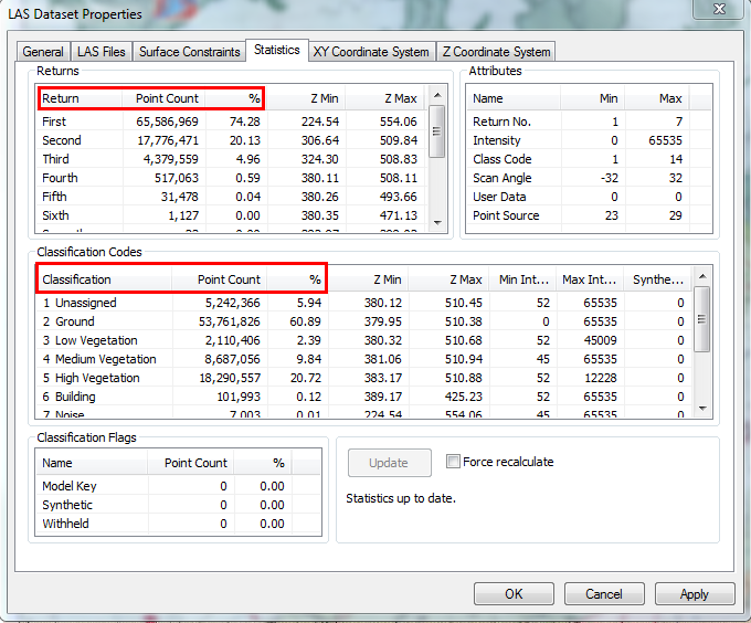
LiDAR data consist of multiple "Returns" (upper left table): light pulses that bounce back to the instrument. A "return" is a specific arrival at the instrument from a single laser pulse.  For each pulse, these are classified by whether they return quickest ("First returns") or at successively later times (Second, Third, Forth, etc.).  As shown in the statistic table, the number of returns from laser pulses diminishes with time - ~75% of all returns are first returns whereas fewer than 5% are third returns.

During post-processing, most returns are assigned a standard Classification Code (middle table) based on the origin of the return.  The distinction between return number (i.e first, second, etc.) and Classification code is important - it is easy to understand that for partially vegetated areas some first returns will come from the ground whereas others will from the tops of trees.  We are interested in returns that are classified as ground returns - coded 2 - but note that Code 9 are water returns and Code 3-5 are vegetation returns.  For this dataset, points with ground returns are most abundant (~61% of all data) but note that 6% of the points had returns that were not classified ("unassigned" - Code 1) and ~32% of the points had returns from vegetation (Codes 3, 4, 5).

The strength or Intensity of returns (middle table) are also measured (on a scale of 0 to 65,535) - some pulses come back strong, some weak.  Strong returns come from highly reflective surfaces, weak from surfaces that absorb some of the laser pulse.  Minimum and Maximum Intensity measurements are listed for each classification.

6. Drag the Nueces LAS Dataset from ArcCatalog into a blank Arc Map window.  You have just loaded the entire point cloud, all ~88 million points.

7. The ArcMap window shows only the outline of each of the four data tiles (this keeps redrawing times reasonable) until you zoom to a specific area.

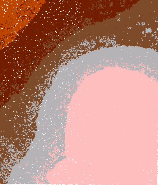
8. Zoom into the lower right corner of the lower right tile.  Your screen should look like the image below but without the pink, which on your map will be white.  You are looking at a two dimensional view of a point cloud, color coded by elevation - the ArcMap table of contents shows the range of elevations (in meters) represented by each color.  White is an unfortunate color choice for an elevation interval because it also represents background areas of no points.  Choose an unused color (I chose pink) and replace it by changing the symbology of the top-most point in the table of contents.

9. Open the LAS Dataset toolbar (Customize>Toolbars>LAS Dataset), which contains a variety of options for viewing and manipulating point clouds.



If the toolbar is grayed-out, you will have to turn on the Spatial and 3D analysts extensions, as indicated in the step 2 above.

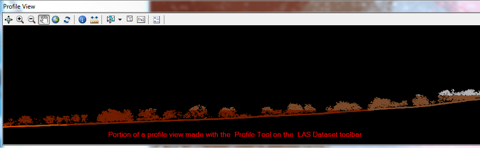
10. Want to see something astounding? Use the Profile Tool (second from right on the LAS Dataset toolbar) to construct a short vertical profile (a cross section) through the point cloud.  A tool tip, visible when hovering the mouse over the tool, explains how.  These are unfiltered points, so we are viewing returns irrespective of Code Classification.  We won't spend much time with this tool but it's just to cool to ignore!
  Explore the other tools on this toolbar - they provide very powerful ways to view and interactively filter LAS point clouds.

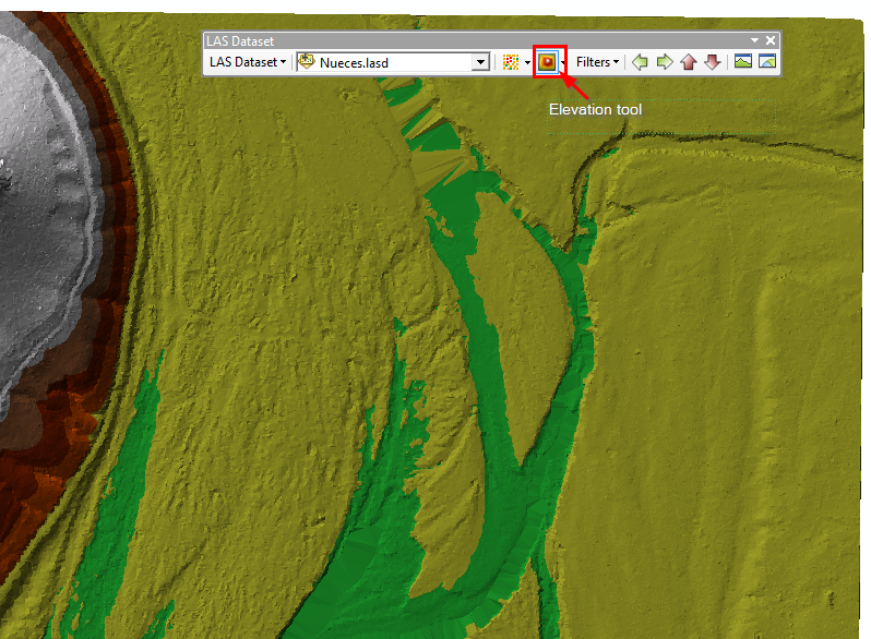
11. Can't resist one more trick with this toolbar... create a surface elevation model (a TIN) with the Elevation tool on the toolbar (see below) by zooming in or out of your Map.

The maps created with the LAS Dataset toolbar are visualizations created on-the-fly, not permanent products.  As such, they are of limited use for analysis.  We would like to create a permanent raster dataset from this LiDAR (vector) point cloud - specifically a high resolution, "bare earth" Digital Elevation Model (DEM; nomenclature varies - LiDAR-derived bare earth rasters are commonly referred to as Digital Terrain Models (DTMs)).  This will require a tool from ArcToolbox.  

12. Using the Search window in ArcMap, search "LAS to Raster" for a the tool needed for this conversion.
13. IMPORTANT - Before running this tool make sure a) that you are zoomed completely out and can see the red outlines of all of the data tiles in ArcMap; b) that the LAS Dataset Toolbar has the "Filters" tool drop-down set to "Ground" and the Point tool drop-down set to "Elevation".  These choices will be recognized by the "LAS Dataset to Raster" tool in ArcTool box if we take care to choose the ArcMap layer as the Input Dataset and not browse to and choose the original LAS Dataset.
     
14. Open the "LAS Dataset to Raster" tool from ArcToolbox or the Search window.  If not already shown, show the Help for this tool. USING THE DROP-DROWN ARROW AND NOT THE FOLDER ICON (see graphic below), select Nueces.lasd as the Input the LAS Dataset

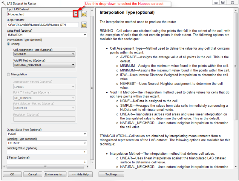
• name your output raster Nueces_DTM, to be stored in your LiDAR folder of Lab_7_data folder
• Value Field is ELEVATION,
• Interpolation Type is Binning with "MINIMUM" (this is a bare earth model...) as the Cell Assignment Type and NATURAL_NEIGHBOR as the Void Fill Method. 
• DO NOT CLICK OK YET -we need to specify the raster resolution (cell size), which requires some thought.  The raster cell size should never be smaller than the point spacing of returns.  As seen in the statistics, the average return spacing is about 35 centimeters. This is for all returns, irrespective of classification.  We are using Class 2 (ground returns) only, not all points, so the spacing for these returns may be significantly greater (3x to 4x greater- not all points will have ground returns) .  A conservative approach for a bare earth DTM is to set the raster cell size to ~ 3 times the average return spacing.  For our data this means about a 1 meter cell size, SO SET THE "Sampling Value" TO 1.
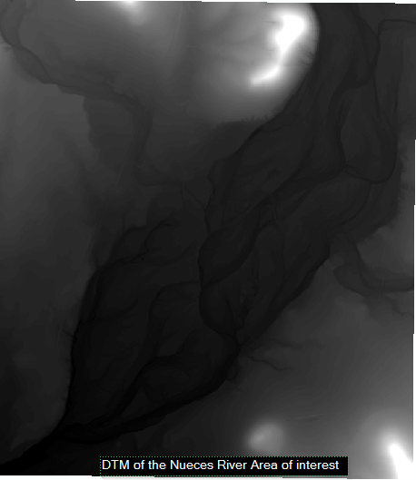
• Z Factor is 1. Click OK. This will take a few minutes...

If all went well your DTM should look like the one below.

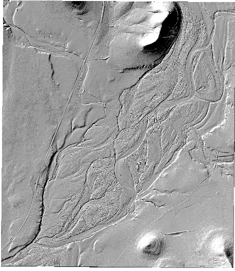
This new DTM will be easier to visualize in shaded relief.

• Using the Search window, find the Hillshade tool in ArcToolbox and create a Hillshade, like that created in Lab last week (Part D).  By changing the symbology Stretch Type to Percent Clip (Min 2, Max 2) you Hillshade should resemble the one below.

9.4 Constructing a Preliminary Map for Field Work

In the interest of time, a preliminary geologic map of the area of interest has been constructed from the LiDAR dataset, 2012 orthophotos, NHD data, and prior knowledge of the geology of the region.  Your task is to add to the map by digitizing the Nueces River channel as it existed in 1996.

1. Open the map document in the Lab_7_data folder and add your DTM and Hillshade to it.  The Rocks and terrace deposits layer contains polygons for the following rock units:

   1. The active river channel: least vegetated, narrowest portion containing the modern river and its point bars

   2. Terrace level 4 (T4): river and stream deposits at slightly higher elevation that the active channel (or stream beds). The hillshade of this unit shows a characteristic plumose texture of downstream diverging rill and elongate lobes formed during flooding of the active channel.  Some of the abandoned subsidiary channels within this unit contain standing water and appear to have been active channels during high flows or floods.

   3. Terrace level 3 (T3): At a slightly higher elevation than level 4 terraces, these deposits are characterized by relatively smooth surfaces that don't appear to have been greatly disturbed or reworked by floods in recent times. Where they border T4 they are densely vegetated by large trees.

   4. Terrace level 2 (T2): Flat smooth surfaces in stream valleys on the NW and SE sides of the Nueces River that are elevated above T3.

   5. Terrace level 1 (T1): the highest relatively flat surfaces in stream valleys and along the Nueces River.  Contacts with bedrock unit Ku are difficult to discern and some of what is mapped as Ku may be T1.

   6. Undivided Cretaceous rocks: At the lowest elevations, this unit includes uppermost Glen Rose Limestone which by weathering characteristics (gentle uniform slopes) appears to be soft, easily weathered marl or claystone. The highest elevations are likely capped by resistant lowermost carbonates of the Devil's River Formation. 

2. Create a Line feature class, "River_1996", in the  "Geology" Feature Dataset of the Nueces_River_2014" geodatabase. 

3. In the ArcMap Table of Contents turn off all but this layer and the 1996 USGS orthophoto.  Using the criteria described above for the present active river channel and by analogy to how it looks in comparison to the 2012 orthophotos, carefully map the outline of the active channel as it existed in 1996.  The procedure will be exactly like the digitizing you did in Lab 4. There are significant differences between the 2014 and 1996 channel that may reveal where buried channels might be today. 

9.5 Printing Field Maps

1. Layout your finished map to fit on 8.5x11" paper, place a UTM grid on top of it and print color copies for use in the field of:
   1. The hillshade with unit contacts (but not rock and terrace units) and the 1996 channel outline clearly visible
   2. The 2012 orthophoto overlain by 70% transparent Rock and terrace units, with the outline of the 1996 channel on top.

 Bring these maps with you on the field trip.

9.6 Trimble Nomad and ArcPad v. 10

GPS data collection using the Trimble Nomad units is done with ArcPad software.  ArcPad is a streamlined version of ArcGIS that is equipped with very easy to use GPS capture tools.  ArcPad 10 is installed on the classroom computers and our field data collection units.  Version 10 is a major revision from earlier releases.  Before getting a little ArcPad practice, we first need to convert the ArcGIS map document file into an "ArcPad Project".  An automated tool exists to do so, which converts most rasters to jpeg images, the geodatabase to an ArcPad exchange format database (.AXF), and makes data entry forms from the domains for each Feature Class.  We can "check out" the empty Feature Classes for editing then, upon return, "check in" the same, permitting the software to automatically update the geodatabase!

An important note about ArcPad versions:

• ArcPad 10 represents a significant departure from earlier versions (i.e. 8.x and below).  "ArcPad Projects" created for ArcPad 10 will not run on 6.x software, and vice-versa.  The ArcMap toolbar for creating ArcPad projects in versions of ArcGIS 9.1 and higher contains separate tools for creating ArcPad 8.x and 6.x (or lower) projects.  It is thus important to know which version of ArcPad is installed on your field data collection units.  Our Trimble Nomads and Xplore tablet PCs are currently running ArcPad 10, as are the computers in the lab. 

A. Preparing the Map Document for ArcPad (version 10).

1. Open your map document.
    
2. Switch to Data View mode (if you're in Layout mode) and zoom to your Hillshade layer.  This is an important step!
    
3. Make sure the "Point" and Rock Unit contacts Feature Classes are present in the Table of Contents of the map.  These have coded-value domains already built that will allow use of ArcPad data entry forms.  These are the files you will populate with GPS measurements.
    
4. Change the symbology of these files to colors/symbols that will be recognizable on both a white background and the DOQ.  Red works well, as does light blue.  This is much easier to do now than later in ArcPad.
    
5. If not already on. Turn on the ArcPad Data Manager toolbar (Tools>customize...) shown below.
    

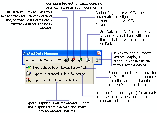
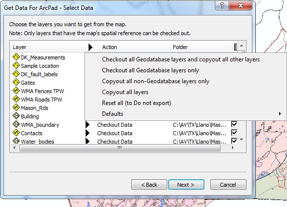
6. On the ArcPad toolbar, click the "Get Data for ArcPad" button.
    

7. Click the black arrowhead to the left of your "Points" Layer and choose "Checkout for disconnected editing in ArcPad>data based on defined extent".  Do the same for the Rock Unit contacts layer.
8. For all other vector layers choose "Export as Background data (to AXF layer)>Make Read Only"
9. Do not export the raster files.
10. Click Next.

12. The next window, "Select Picture Options", is not applicable to this project; Click Next.
    
13. The final window lets you set the spatial extent (current display extent or full extent of the layers), lets you select whether to limit the fields to those that are visible in the attribute tables and the features to those specified in the layer's definition query, lets you specify a name for the folder that will store the data, and lets you create an ArcPad map file (the equivalent of an .mxd file) for the data, as shown in the "Get Data For ArcPad" screen capture below.
     
14. Enter a name for the folder, e.g. "ArcPad_Nueces_XX" (where XX are your initials) and a Map Name that includes your last name or initials (e.g. NuecesRvr_XX).
     
15. Making sure first that your display shows the entire area of interest (i.e. you are zoomed to the area of interest), make the selections shown in the figure below, setting the "Where do you want the folder to be stored?" to an appropriate location on your network storage space.

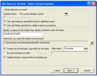
16. Click Finish and wait for the data to be created.
     
17. With help from Ali, transfer your new "ArcPad_RR_XX" folder to your Trimble Nomad (these will be shared, but each partner can load a project). The Nomad units have a folder called "My Documents" that should be used for all ArcPad data and files.
    
    
18. Print a color copy of the PDF file "ArcPad Quick Reference", in color, from All Programs>ArcGIS>ArcPad 10>Help>ArcPad Quick Reference.  You will find this exceptionally useful for Part B of this lab, and for the field trip.

PART B  

Practice with ArcPad in the field

9B.1 Using ArcPad - some practice with the basics

Editing in ArcPad is, in most ways, much simpler than Editing in ArcGIS.  The basic concept is the same in both - data are entered into a file that is open for editing.  Below are a few of the basics.  A complete description of the software can be found in the ArcPad 10 folder in the class folder.

1. On a classroom computer, open ArcPad 10 from the Start Button>All Programs menu in Windows.
    
2. Click the folder button at the top of the ArcPad window and select  "Open Map", then browse to your ArcPad map file, the one with the ".apm" extension, in your "ArcPad_RR_XX" folder.
   
   
3.  Five toolbars are immediately available (called Main Tools, Browse Tools Edit Tools Quick Capture and Navigation), though only one at timeis displayed  (this saves real estate on small screens).

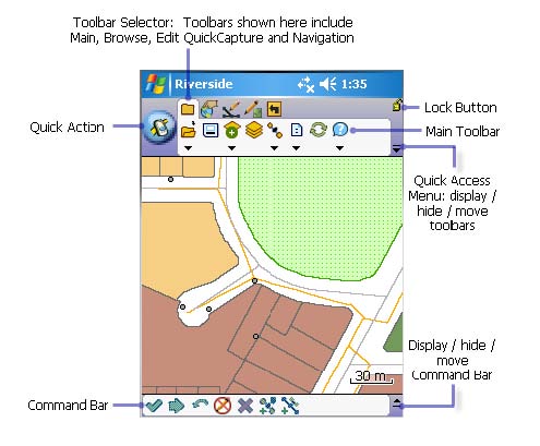
4. Click the Main Tools icon (on the left in the figure above) and then select the Layers icon to open up a Table of Contents, like that on the left below.  The diagram on the right, from an earlier version of ArcPad, has many of the icons labeled.

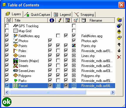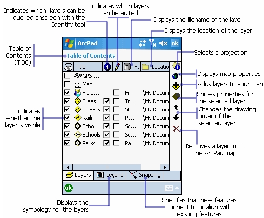
5. The check boxes on the left in the "eye" column turn layers on and off for viewing.  The check boxes in the "pencil" column turn layers on and off for editing.  This is similar to setting the "Target" of the editing toolbar in ArcGIS, except that in ArcPad more than one layer can be open for editing at a time.  In the Table of Contents to the right above, none of the layers are open for editing. In the table of contents on the left above three layers (Point, Line, Polygon) are open for editing. Finally, the check boxes below the Info icon (i) make layers available for query.  Layer Properties can be accessed by an icon on the right, as can other options denoted by icons that should be familiar from ArcMap.  The column with the "rocket ship" icon at the top is the QuickDraw mode; checking boxes here allows the different layers to be drawn to different "coarseness" so they will render quicker on screen.  The QuickDraw mode is accessed from the Editing Toolbar.

6. Turn on the "Point_XX" layer for editing and close the Table of Contents.

7. Turn on the Edit toolbar by selecting it from top row of icons, as shown below.

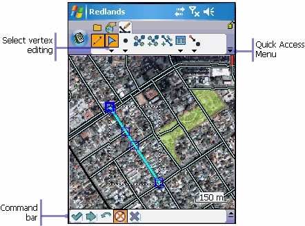
8. The function of the edit tools are shown in the figure below.  This is the most important toolbar for the field work this weekend.  Learn it.

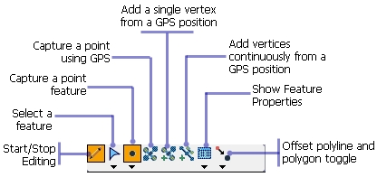
To add a point to the map, Click the pencil tool, select the layer you want to edit, click the "Capture a point feature" button, (Capture of polyline or polygon features, if open for editing in the TOC, can be selecting from the drop-down menu below the "capture a point" feature icon). Then click a location on the map.  A data entry form should then open, allowing you to select the feature name from a drop down list.

To do outdoors: To add a GPS location as a point, click instead the "Capture a point using GPS" button. (When the GPS is active this button is not grayed-out.)

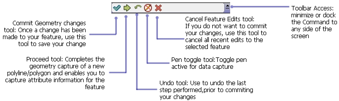
9. To add a line, click the Pencil icon, select the polyline feature class you want to edit, click the drop-down arrow below to the "Capture a point feature" button, and select "Polyline".  Click on the map where you wish to place a polyline vertex, click and drag on the next spot where you want a vertex, and continue this process until finished.  The line is not completed until you click the "Proceed or complete feature" button at the bottom of the ArcPad window (shown below).

10. To do outdoors: To add GPS vertices to a polyline, as above, click the "Capture a polyline" button (beneath the capture a point button), click the "Add a single vertex from a GPS position" button and continue clicking this button every time you want to add a vertex to the line.  To finish the line, click the "Proceed or complete feature" button, the green arrow icon. The line is not completed until you click the "Proceed or complete feature" icon.
    
    The GPS must be activated before the GPS buttons are available. 

11. A similar procedure is used to capture polygon vertices with and without GPS.

12. You can delete features by selecting them with the Arrow button (shown above) and then clicking the "Edit vertices" button.

13. Practice adding and deleting lines, points and polygons to the map.  Name the features test1, test2, etc. so that, if needed, you will be able to recognize and delete them later.

14. Browse the ArcPad manual in the digital books folder, particularly the sections on editing.  Download and print the ArcPad Quick Reference page.

15. Before loading your ArcPad folders to the field GPS units, clear each of your test features, or don't save your project after editing.

9B.2

1. Before our field trip, you need practice using ArcPad with a GPS. An ArcPad project for the Main Building area, identical to the ArcGIS project you constructed in Lab 6, is loaded on all instruments.  Take your instrument outside, open the Main Building project, and practice capturing lines, points and polygons using the ArcPad GPS tools described above.

2. Specifically, capture the features listed and labeled in the photo below.

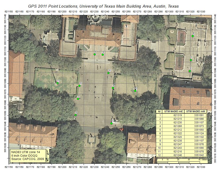
• Points: Points at the two flagpoles.
• L1, L2, L3: Polylines with at least 3 GPS vertices at the edges of sidewalks.
• P1, P2: Polygons outlining grass areas - capture the vertices of the 4 corners with GPS. s - capture the vertices of the 4 corners with GPS.

You're done.