|
I. Goal
Assess the volcanic hazards associated with Mount Rainier, a dormant
but recently active volcano in the Cascade Range of Washington, and compare the results
with the US
Geological Survey (USGS) Open File Report 98-428 "Volcanic Hazards From Mount
Rainier". We will do so using data stored in a variety of
different formats (shapefile, coverage, .e00, geodatabase feature
classes, and raster .grd), providing familiarity and practice with
commonly used data types.
II. Problem
At 4939 meters (14,410 feet), Mount Rainier is the highest peak in the Cascade Range
and one of the highest mountains in the continental US. It is a dormant but recently active volcano that also hosts
the largest glacier in the lower 48 states. The combination of potential
volcanic activity, high topographical relief, and an ice cap pose
significant natural hazards, especially during an eruption.
Whereas magmatic flows from an eruption may be fairly limited in extent,
tephra fall and lahar flows could affect populations far from the
volcano. What areas could be most
affected by an eruption of Mt. Rainier? How many people could be
directly affected? Working with some basic constraints and
assumptions, existing digital data can be used to address these
questions. Furthermore, we can compare our results to ground-truth data
of the USGS to gauge the utility of our hypothetical approach.
III. Data
Data for today's lab comes from three sources:
- The
Washington State Department of Natural Resources GIS web site: county boundaries, rivers, the
Mt. Rainier summit, and digital elevation models (DEMs) files;
- ESRI ArcGIS 9 data disk: a file of populated places in Washington, with 1990 census numbers;
- USGS: A PDF of
USGS OFR 98-428, from which
tepha, lahar and volcanic flow hazard areas were extracted and
converted to feature classes. The extraction and conversion
process is documented in the metadata for the files.
Metadata for all of the files
can be viewed in ArcCatalog. A copy of OFR 98-428 (and the plates and figures
within it) is available in the "Lab_10_data" folder.
The "Lab_10_data" folder and sub-folders contain files with the following
formats:
- ArcInfo Interchange (.e00) files - DEM rasters, in Arc
GRID format, for parts of the
counties surrounding Mt. Rainier:
- king_co - King County, WA
- pierce_co - Pierce County, WA
- yakima_co - Yakima County, WA
- kittas_co - Kittitas County, WA
- lewis_co - Lewis County, WA
- thurst_co - Thurston County, WA
- Coverage
- County - a coverage of counties in the state of
Washington
- Shapefiles for the following features:
- all_cities_StatePlaneft - the towns and cities of Washington
(as points);
- Mt_Rainier - the summit of Mt. Rainier (a point);
- wa_rivers_arc - the major
rivers of Washington (lines);
- WA_State - the State of
Washington, (polygon);
- Area_of_Interest2 - a rectangular defining the area
of interest (AOI) for this lab (polygon).
- Geodatabase Feature Classes (USGS hazard files):
- flow_area - hazard area for lava or ash flows (polygon);
- lahar_polygons- within the Feature Dataset
"Lahars", these are hazard areas most likely
affected by lahar flows, separated by likelihood of flow recurrence and
size (polygons);
- Tephra_10cm - hazard areas for 10 cm of tephra
deposition, displayed as annual percent probabilities (polygons);
- Tephra_1cm - hazard areas for 1 cm of tephra
deposition, displayed as annual percent probabilities (polygons).
Copy the entire Lab_10_data folder to your storage space now. Do
not copy individual files and subfolders - the integrity of some of the data will be destroyed if you do so. If individual raster
files or coverages must be copied, do so with ArcCatalog, not with
Windows Explorer.
An MS Word document with the questions for this lab can be found in the
Lab_10_data folder.
IV. Procedure
The procedure involves the following general steps:
- Convert interchange files into grid (DEM) files. Mosaic the
individual DEM files into a single DEM file;
- Select rivers that that have headwaters on Mt. Rainier, and build a
new shapefile from these data;
- Specify hazard zones for both tephra fall and lahar flows. Select
towns and cities that would be affected by these hazards;
- Calculate the area affected by lahars and tephra fall and compare
these estimates to those to those of the USGS. Also calculate the total
population that would be affected by a volcanic eruption at Mt. Rainier.
We begin first by exploring the data.
A. Explore the Data
- Open ArcMap and create a new, empty map.
- Load the State, County, and Area of Interest polygons, the rivers, and the Mt. Rainier and cities point
shapefiles.
- Symbolize these shapefiles so that the Counties are hollow, and
the State is visible beneath them. Also make sure that your rivers, area
of interest, cities, and Mt. Rainier are symbolized appropriately.
Your map should look similar to the one below:
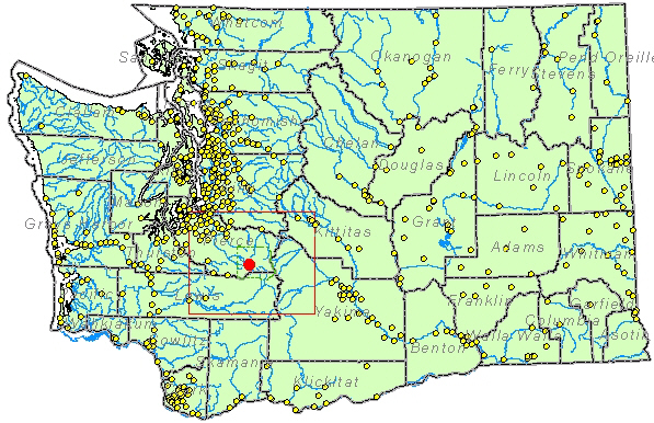
Figure 1. Cities (yellow), counties, rivers and
the state of Washington showing the location of the area of interest
(red box) and Mt. Rainier (red dot).
- Use the add data button and try to load the DEM data from the
"WA_DEM_E00" folder.
You will notice that ArcMap does not
recognize any of the files contained in the folder as data. We will
need to fix this.
B. Converting Interchange Files into "Useful" Files
If we open the "WA_DEM_E00" folder in Windows
Explorer, we see that the files within it are of the type ".e00". Data in .e00 are in an ArcINFO
Interchange file format. These are simple ASCII files that can be opened
and viewed using any common text editor (i.e. wordpad, notepad; see Fig.
2). This
format is commonly used to make coverages and raster Grid files
available online, because it compresses the file size, which helps both
with hosting large amounts of data and downloading large files. It
also provides a way of maintaining file integrity. Coverages contain hidden files as part of their data
structure that might be lost during copying without an interchange
format.
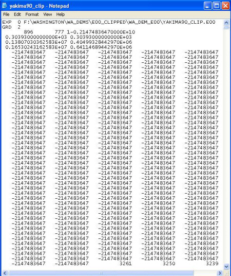
Figure 2. An .E00 DEM file displayed in Notepad
- Open ArcToolbox, and select the "Coverage"
toolbox. Then select the "Conversion" toolbox, and choose "To
Coverage". Select the "Import from Interchange File" to open the
tool.
- Leave the "Feature Type" as AUTO. Under "Input
Interchange File", click on the folder to the right of the entry
area and select one of the .e00 files in the WA_DEM_E00 folder. Make
sure that the "Output Dataset" is being mapped to the same folder,
and that the name is the same as the file being converted. Then
click "OK".
- Do the same for the remaining .e00 files.
If you get an error message, try again with a shorter file name for the "Output Dataset".
Inexplicably, the default file name is sometimes greater than 13
characters and the conversion fails as a result. The same error can
result if any of the names in the path to the output file exceed 13
characters, contain a space or contain a special character (e.g. period,
asterisks, etc.). Remember this bug - it may be useful in later
project work.
- Add the new files to your map, placing them at the bottom of the table of contents.
Question 1: What is the coordinate system of the DEM
data?
Question 2:What are the horizontal and vertical units of the raster data? How do we know this?
Question 3: What are the pixel depth, type, and size for the raster datasets?
|
C. Creating a Mosaic of Raster Data
If we wanted to modify the symbology of our DEMs, we would have to
symbolize each layer separately. This is
inconvenient and tedious, but more importantly usually leads to differences in how
identical elevations in different DEMs are
symbolized. Unless the highest and lowest elevations for all DEMs
are identical, the same color ramp (see below) applied to each file will
yield different colors for the same elevations. One way to avoid this
problem is to mosaic the
individual DEMs to create a single DEM that contains all of the data (a
second
way is also explained). To
do this, we will again need ArcToolbox.
- Before getting too far along, create a new, empty folder in your
"Lab_10_data" folder entitled "My_Data". This folder will be useful for
saving new layers and shapefiles that you create throughout the lab.
- To begin the mosaic, got to ArcToolbox, Select "Data Management Tools" and then "Raster", since we
are dealing with raster datasets.
We now have a couple of options. We can use either the "Mosaic" or the "Mosaic to New Raster" tool. "Mosaic"
is useful if we want to add additional raster data to a pre-existing
raster dataset. While this is often useful, we would rather create an
entirely new
raster that we can give a new name.
- Choose the "Mosaic to New Raster" tool. Navigate to
the folder that contains your raster datasets, highlight them all
(hold the shift key down and select the first and last file in the
list), and hit "OK". Select the "My_Data" folder as your output
location. Name the new raster in the line labeled "Raster
Dataset Name with Extension". Read on...
We want the spatial reference for the mosaic (the next entry line
in the tool) to be the same as that of the original DEMs. To
ensure this:
- Open the "Spatial Reference Properties" window by
clicking on the icon next to the entry box, choose "Import", and
select one of the original DEMs, then hit "OK". This "imports" the same spatial reference
from the DEM to the mosaic.
- Change the "Pixel Type" and the "Cell Size" to match the size
of the original DEMs. Ignore the rest of the fields
and hit "OK".
- The new DEM mosaic is automatically added to our project, and we
can remove the original, single DEMs from the TOC.
The mosaic should resemble the one shown in Figure 3.
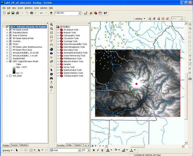
Figure 3 - ArcMap showing Data View of the completed DEM raster
mosaic.
Question 4.When we created the raster mosaic, we were
given the option of changing the cell size. What would changing the
cell size do, and why did we choose to keep it the same? |
D. Selecting Rivers at Risk From Lahar Flows
Lahars are mud-rich debris flows that begin on the steep slopes of
volcanoes when rapid melting of snow or ice takes place. Because all
that is needed for lahars to form is mobile, unconsolidated sediment
(e.g. volcanic ash, lapilli, bombs), steep slopes and lots of water,
lahars can form while a volcanic is dormant if enough rain or melt water
is available. Lahars can, of course, also be initiated by rapid
melting of snow/ice before or during an eruption. Using existing streams
and rivers as conduits, lahars can flow great distances (lahars from Mt. Rainier have
flowed into Puget Sound) and be very destructive. Lahars from Mt.
Rainier are considered the single most significant volcanic hazard in
the Cascade Range. Where are the river valleys that are at
greatest risk from lahars?
Our "WA_river_arc" shapefile contains all of the rivers in the state of
Washington. We are only interested in the ones that drain the slopes of Mount Rainier. These rivers are
the most likely conduits
for lahars traveling away from the volcano, and we would like to select
and isolate them. To select these
rivers it would be useful to have a clearer view of the topography so
that we could, at a glance, identify valleys and ridges. Having a
rendering of the "Aspect" of the topography would help. The
"Aspect" tool derives the aspect, the down slope direction of the
greatest rate of change from each raster cell to its neighbor. We can think of
aspect as the slope direction or, if we
dropped a marble at a point on the surface, the direction it would
roll.
- Open the "Aspect" tool, which is located in ArcToolbox under
"3D Analyst Tools" - "Raster Surface". Our "Input Raster" will be
our DEM mosaic and the "Output Raster" will need an appropriate
name. Again, save it to your "My_Data" folder. The Aspect map
(see Fig. 4)
should makes it easier to visually distinguish drainages, ridges and
slopes, though you may need to change the color ramp to see this
more easily.
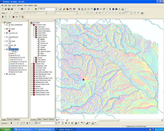
Figure 4 - ArcMap showing Data View of an aspect raster and rivers
in an area of interest around Mt. Rainier (red dot).
- By inspecting the aspect map, identify rivers that
have headwaters on the slope of from Mount Rainier.
- Select these
rivers, use the "Select Features" tool
 on the standard toolbar. To avoid selecting anything but the rivers,
set the "selectable layers" first; this gives you a chance to turn
off the "selectability" of all but the rivers. One way to set selectable layers (we learned another
in Lab 3) is to click the "Selection" tab at the bottom of the TOC, then check on the Rivers
layer and turn off all others, as shown in Figure 5 below.
on the standard toolbar. To avoid selecting anything but the rivers,
set the "selectable layers" first; this gives you a chance to turn
off the "selectability" of all but the rivers. One way to set selectable layers (we learned another
in Lab 3) is to click the "Selection" tab at the bottom of the TOC, then check on the Rivers
layer and turn off all others, as shown in Figure 5 below.
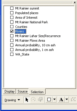
Figure 5. Table of Contents viewed with the Selection
tab active. When checked, only the Rivers layers is selectable by any of
the selection tools.
- Make sure that you have selected each river's full
reach within the Area of Interest.
Question 5. What are the names of the rivers that are
potentially at risk from Mount Rainier lahars?
|
We now want to save ("Export") the selected rivers to a new shapefile.
- Right-click on the "wa_rivers_arc" file name in the
TOC, and select "Data" - "Export Data". Then choose to Export
"Selected Features" and save the file in your "My_Data" folder.
- You will then be asked if you want to add the exported data
to the map as a layer. Select "Yes".
- To remove the portions of these rivers that extend beyond the
Area of Interest, open the "Clip" tool from ArcToolbox (within
toolbox "Analysis
Tools" - "Extract").
- Use your new rivers shapefile (these are the rivers at risk from
lahars) as the "Input Feature", and choose the Area of
Interest polygon as the "Clip Features". Rename the "Output Feature
Class" appropriately, and hit "OK". N.B.
for later work: the "Clip Features" tool will only work if the
clipping polygon and the data you are clipping have the same Spatial
Reference (these do).
Your result should look like Figure 6 below.
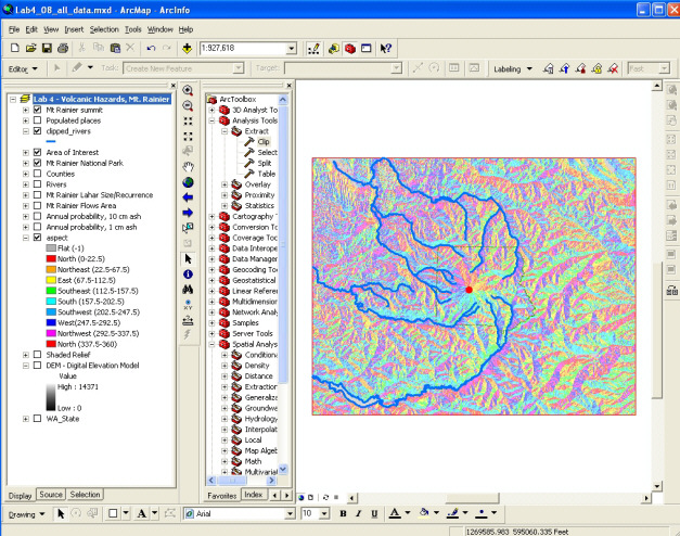
Figure 6. ArcMap Data View of rivers having headwater on the slopes of Mt. Rainier,
clipped to the area of interest, and an aspect raster.
F. Viewing Elevation Data in ArcScene
Another way to visualize topography is with the ArcGIS program ArcScene. ArcScene is for
3D visualization and analysis. You can find it from the Windows "Start
Menu"; it is in the ArcGIS program group.
- Open ArcScene and load your DEM mosaic into
the program.
- Right-click on the mosaic layer title in the
TOC, and select "Properties". Under "Properties", select the "Base
Heights" tab and click on the radio button next to "Obtain heights for layer
from surface". Make sure that the surface that you're getting the
heights from is your DEM mosaic . Then click on "Raster Resolution" and
make sure that the cell size is the same as your original surface. Also
make sure that the "Z Unit Conversion" is 1 and hit "OK".
Your previously flat DEM should now be a 3D surface (Fig. 7).
- Now add the "WA_rivers_arc" shapefile and do the same thing, making sure that the base heights are
being computed from the DEM mosaic . Under the "Symbology" tab for your
DEM mosaic (again in the Layer "Properties" window), select
"Stretched" with the "Stretch Type" as "Minimum-Maximum". Set the "Color
Ramp" to "Brown to Blue Green Diverging, Dark" (a right-click on the
color ramp selector will list the color ramp names) and hit "OK".
- Under "Scene Layers" select "Scene Properties" and go to the "General" tab.
Change the "Vertical Exaggeration" (VE) so that the topography becomes more
apparent (in this case, a VE of 2 should be sufficient).
- We can now see which rivers drain the slopes of Mount Rainier. Use
the "Identify" tool to check these rivers against the ones that you
selected using the aspect raster in ArcMap.
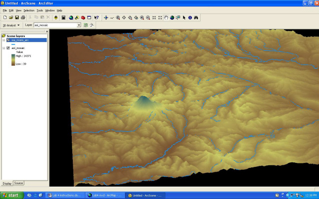
Figure 7. ArcScene image of the DEM mosaic, rendered
with a color ramp, and the rivers file (blue lines). Note that the
display shows all rivers, not just those with headwaters on Mt. Rainier.
Make a screen capture of your ArcScene map
and attach it to your lab questions.
|
G. Hazard Assessment
As mentioned at the beginning of the lab, there
are two major hazards associated with Mount Rainier: tephra
fall and lahar flows. The area affected by tephra fall is
directly related to the distance from the summit of Mount Rainier (assuming the eruption
is from the summit, not from a lateral
blast). Large tephra fragments are capable of causing injury or death by
impact, and may be hot enough to start fires where they land, but do not
usually come to rest beyond 10 km (~6 mi) from the vent of the volcano. Small tephra is hazardous when accumulation on the roofs of buildings
exceeds 10 cm (~4 in), potentially causing collapse, and can extend up to
100 km (~60 mi) from the vent.
Lahars are a different matter.
Past lahar flows from Mount Rainier have typically been 10-40 m (~30-120
ft) thick, and have traveled hundreds of kilometers, some extending
out into Puget Sound. Areas affected by lahars will be near rivers
draining Mount Rainier, so what we would like to do is identify areas
along the rivers/streams at risk from lahars of different size.
G.1 We begin with tephra hazards. We would like to create two,
superimposed, concentric circles, centered on the summit of Mount
Rainier, with radii equivalent to distances potentially affected by
large and small tephra fall. To create these circles we will use a
"Buffer" tool. Because we want to create two superimposed circles, we can use the "Multiple Ring Buffer", which can be found in ArcToolbox under "Analysis Tools" - "Proximity".
- Open the Multiple Ring
Buffer too. Under "Input Feature Class" choose the "mt_rainier" point shapefile, and name the "Output Feature Class" appropriately. Now, add
the two distances mentioned above (6 mi, 60 mi), making sure that the buffer unit is
set appropriately (for this exercise, we will use miles). Leave the
"Field Name" blank, and choose "None" as the "Dissolve Option".
Now hit "OK".
This
creates two superimposed circles (as opposed to concentric rings), which
can be use to calculate the areas of the different tephra hazard zones.
- Symbolize the newly created buffer layer by "distance" (see Fig.
8).
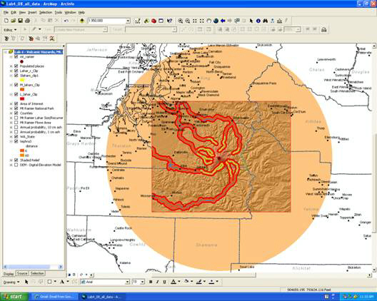
Figure 8. Buffers of 6 miles (dark orange) and 60 miles
(light orange) away from the summit of Mt. Rainier.
We can now calculate the area of the newly created tephra hazard
zones:
- Open the "Attributes" window of the buffered layer.
"Right-click" on the "Area" tab, and choose "Calculate Geometry…". A
warning dialogue box will pop up asking you if you would like to
continue. Click "Yes". Under "Property", select "Area", and make
sure that the "Coordinate System" is set to the coordinate system of
the data source. Under "Units", select "Square Miles", and hit "OK".
Do the same for the "Perimeter" tab, setting the "Property" to
"Perimeter" and the "Units" to "Miles".
Question 6. What are the areas and perimeters of the
buffers that you created for the tephra fall zones?
|
G.2 Lahars can be considered as small, medium, or large. These categories are
outlined below:
Table 1. Lahar flow size, width, distance traveled
| Size |
Width |
Distance from Summit |
| Small |
1 km (0.6 mi) |
20 km (12 mi) |
| Medium |
2 km (1.2 mi) |
throughout AOI |
| Large |
4 km (2.4 mi) |
throughout AOI |
We can use the same buffer tool to identify lahar
hazard areas, only this time we will use the clipped rivers shapefile
instead of the Mount Rainier summit shapefile. Since the lengths of the
lahar events differ, we will use the "Buffer" tool rather than the
"Multiple Ring Buffer" tool, and create separate shapefiles
for lahars of each size category.
- Open the "Buffer" tool, and set the "Input Features" to your
clipped river shapefile. Appropriately name the "Output Features
Class". Set the "Distance" to "Linear Unit", and make it equal to ½
the width of the lahar category that you are creating a buffer for.
Set the "Dissolve Type" to "All", and hit "OK".
- Repeat this process for the other two lahar categories, and
symbolize the new buffer layers appropriately.
Notice that this new shapefile extends throughout the area of
interest. The Small Lahars only travel 12 miles from the summit (see
Table 1). We want to clip these features to an area around the
summit of Mount Rainier limited to this distance.
- Create a single buffer using the Mount Rainier summit point as
your "Input Features", and name the "Output Features Class"
appropriately. Then set the "Distance" to "Linear Unit" and set the
value to "12 miles, and hit "OK".
- Now use the "Clip" tool (ArcToolbox - "Analysis Tools" -
"Extract" - "Clip") to clip the Small Lahar shapefile to the 12 mi
radius from Mount Rainier. Also make sure to clip your Moderate and
Large Lahar shapefiles to the Area of Interest.
To calculate the areas of the Lahars, we will need to add a new field to the
Attributes Table of these layers.
- Open the "Attributes Table", and
under "Options", choose "Add Field…". Name the new field "Area", and
under "Type" choose "Long Integer". Hit "OK".
- To calculate areas for each of the lahars, open the attribute table
again, right-click on the new "Area" field heading, select "Calculate Geometry", choose "Area" under the
"Property" dropdown menu, and "Square Miles" under the "Units"
drop down menu.
Question 7. What is the total area affected by Small,
Medium, and Large lahars? Give your answer in the form of a table,
clearly showing the sum of all of the lahar types.
|
H. Hazard Assessment, At Last
Remember that the ultimate goal of this exercise is to assess the
population affected by a volcanic event at Mount Rainier. We can now
select the population centers (cities) affected by tephra fall and lahar flows using the layers that we have created.
- Use the "Select by
Location" tool located under the "Selection" menu to select cities that
"are contained by" your buffered Larger tephra layer. Open the attribute
table for the cities layer, right-click on the field heading for the
population field (Pop2000), to find statistics on the selected cities. Record what
is needed for Question 8 below. Do the same for the small tephra fall
layer, and for the Small, Moderate, and Large Lahar features.
Question 8. What is the total populations affected by
large tephra fall? Small tephra fall? Small lahar flows?
Moderate lahar flows? Large lahar flows? (Make a table to
answer this question). |
- Load the USGS layer files to your map (note: by
loading the layer files and not the feature classes these layers
will be symbolized for you). An explanation of what these layers
contain can be found in their metadata (examine in ArcCatalog) and
from the USGS Open File Report 98-428 (contained in the lab_10_data
folder).
Question 9.Using the USGS dataset, what is the area (in
square miles) affected by large tephra fall? Small tephra fall? Small Lahar flows? Medium Lahar flows? Large Lahar flows?
How do these areas compare to the areas that you calculated?
Construct a table to show these comparisons.
Question 10. What other criterion do you think that the
USGS authors used to create their hazard assessment?
|
|
To Turn In:
1. The answers to the lab questions.
2. A screen capture of your ArcScene map.
3. A map of your hazard assessment within the Area
of Interest. Include:
a. the Mt. Rainier Summit;
b. clipped rivers;
c. lahar feature classes;
d. tephra feature classes;
e. cities affected by the volcanic hazards
Make sure to symbolize the layers appropriately, and to insert other necessary map
elements. |
You're Done!
|
 |