|
4.0 Objectives
In this lab you will learn to:
- Georeference an image;
- Create a geodatabase, associated domains and
feature classes to store digitized features of a geologic
map;
- Digitize in heads-up mode, construct a topology, and edit features.
4.1 Framework
Three of our next four labs focus on the geography and
geology of the Bastrop Quadrangle near Bastrop, TX, our
weekend field trip site for collecting field observations.
The Bastrop Quadrangle encompasses parts of Paleocene and Eocene formations of the
upper Gulf Coastal Plain, where erosion has exposed very
gently southeastward dipping strata, producing rock
unit bands that young toward the Gulf (Fig. 1). Our focus is
on the geology of the area near the town of Bastrop,
specifically the NE quarter of the Bastrop Quadrangle (Fig. 2).
Here, as elsewhere along the Colorado River, Tertiary rocks
are unconformably overlain by Quaternary gravels, and by
more modern terrace deposits and alluvium near the present
river course. These so-called high gravels, which
occur well outside of and above the modern river floodplain,
can provisionally be separated into a few different units on
the basis of differences in elevations. These
relationships are well illustrated in the geologic map of
the wider region contained in your Lab 4 & 5 data folder.
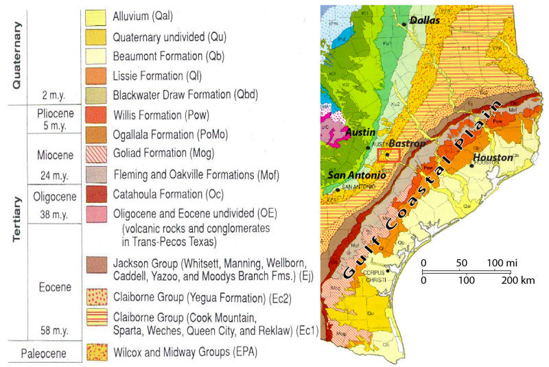
Figure 1. Generalized geologic map of the Texas Gulf Coastal Plain,
modified from a Texas Bureau of Economic Geology postcard. Rock
unit colors not contained in the explanation are Mesozoic or older.
The orange box shows an area centered on Bastrop
contained in Figure 2 below.
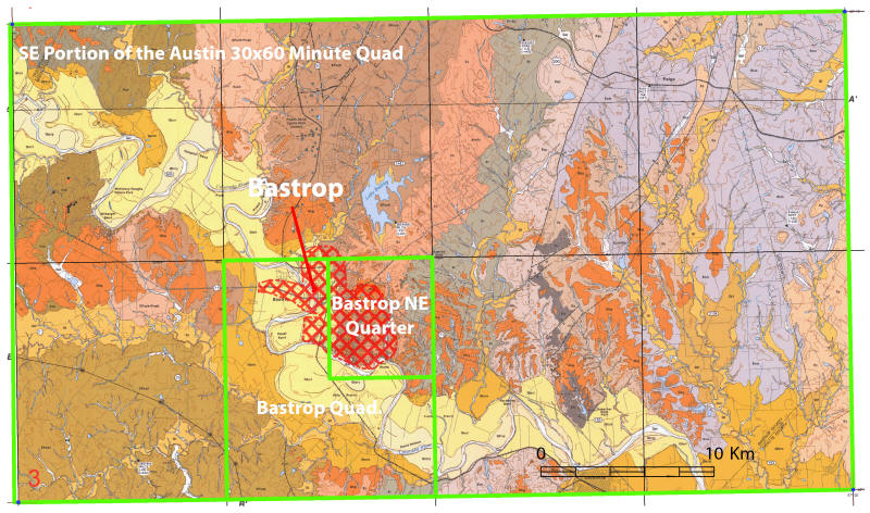
Figure 2. Geologic map (from Collins, 2008) of the SE portion of the
Austin 30x60 minute quadrangle, showing the outlines of Bastrop and the
1:24,000 Bastrop Quadrangle. Our focus is on the geology of the NE
quarter of the Bastrop Quandrangle, also shown. This map and
an accompanying explanation are in the Lab 4&5 data folder.
Our first task, to be completed in this and the following lab (Labs 4
and 5), is to create a vector geologic map of a portion of the NE
quarter of the Bastrop Quad. using a few provided shapefiles and lines
you will digitize from an image of the published (but uncolored) geologic map. Once
completed, this vector map can be used as a base layer for collecting
and edit geologic data during our field trip. The geologic map is most useful when
displayed with other base map layers (roads, contours, creeks, lakes, etc.)
that give it context. Base map feature classes, to be organized
and symbolized, are also provided for this purpose. In Lab 7 we
will generate a highly detailed shaded elevation layer from
airborne LiDAR measurements that can also be displayed with these vector base
map layers.
4.2 Data
Data (and metadata) for this lab are found in the
Lab_4_and_5_data folder in
the network class folder. They include:
- A jpeg image of the published 1:24,000 scale geologic map
of the Burnet Quadrangle.
This image was created from a PDF file of "OFM108: Geology
of the Bastrop Quadrangle, Texas" provided by the Bureau of
Economic Geology. The image does not have an accompanying world file.
You will create one by georeferencing.
- Map Boundary
shapefiles:
- Bastrop Quad. - polygon of the
quadrangle to use for georeferencing
- Area
of Interest - polygon of the NE quarter of
the Bastrop Quad. to be used during
digitizing
- Infrastructure shapefiles:
- Bastrop Co. road centerlines, c. 2015 -
from Bastrop Co. GIS file
- Hydrography shapefiles created from the National
Hydrography Dataset (NHD):
- NHD areas - Polygon file of water
bodies, principally the Colorado River
-
NHD flowlines - Creeks and drainages too
small to show as areas
- Hypsography shapefile:
- 5 m elevation contours were created from
a 1 m LIDAR DEM that you will create in a
later lab
- Geolines shapefile:
- Lines digitized from the NE portion of
the "Geologic Map of the Bastrop Quad.".
About 1/3-1/2 of the geologic contacts have
been digitized; you will digitize the rest.
- USGS 24K Digital Raster Graph of the Bastrop quadrangle.
This is a scanned and georeferenced version of the original
paper map for this area.
- Six-inch(!) resolution
orthophotos of the Bastrop NE quarter quadrangle, from
TNRIS. These are contained in a zipped folder and
comprise, in total, about 500Mb. You will not need
these files for digitizing but they will be useful later.
To complete this lab and Lab 5 you will do the following (in order):
-
Georeference and rectify the geologic map
image
-
Create a Personal Geodatabase
-
Import the Bastrop shapefiles into the Geodatabase
-
Create a
Geology Feature Dataset with a spatial domain that
encompasses the area of interest and import the Geology shapefiles
-
Create
an empty line feature class within the Feature Dataset with the following fields and domain values:
-
a) Exposure (exposed, inferred, covered)
b) Type (fault, contact)
c) Downside (down-thrown side of fault - N, NE, E, etc.)
-
Creates
domains for each field and attach the domains to the
feature class -
Create a map boundary from the map area polygon using
the Feature to Line tool; Append this feature to the line
feature class
-
Digitize geologic unit contacts -
Create a contact line topology
(END OF LAB 4) -
Clean the line feature class of topological errors
(BEGINNING OF LAB 5) -
Create attribute
and symbolize geology polygons
-
Add and symbolize base layer feature
classes (roads, contours, streams, lakes, etc.) -
Add and symbolize geology feature classes -
Label geology polygons and point features
-
Layout and print a map -
Answer and turn in any questions and your layout.
4.3 Procedure
4.31 Georeferencing
-
Copy the Lab_4_and_5_data folder to your network storage.
-
Within your Lab_4_and_5_data folder, create a new folder called
My_Data.
-
Open ArcMap with a new, empty document.
-
Add the BaseVectorLayers>BoundingBox>"BastropQuad_NAD83UTM"
and "Area_of_Interest"
shapefile to the map.
The spatial reference for these files is UTM14N,
NAD83.
-
Add the geologic map image,
"OFM0108-QAd9089_Bastrop.tif". It is not yet
worthwhile to created pyramids for this raster - answer No
when asked.
-
As indicated by a warning
window, this image does not have a spatial reference; the
spatial reference is said to be "undefined".
-
Georeference the geologic map image to the "BastropQuad_NAD83UTM"
shapefile, which has corners that precisely align
with the dashed crosses in each corner of the map image. The
picture below shows a link from the NW corner of the map
image to
the NW corner of the Quad. shapefile.
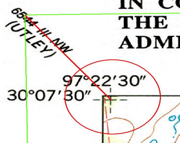
Figure 3. The NW corner (dashed cross) of
the geologic map image is connected to its proper location
at the NW corner of the quadrangle outline (green) via a
displacement link created with the georeferencing toolbar.
Consult the lecture notes and the
Georeferencing
Software Tip for details. For further details on
georeferencing, see pp. 317-322 in the digital book "Using
ArcMap" in the class folder (\Digital_Books\ArcMap\Using_ArcMap.pdf).
Also Search ArcGIS Help for "Georeferencing a raster dataset" and "Fundamentals for georeferencing a raster
dataset".
Watch a
short video
of part of the georeferencing process (with a different
geologic map).
-
Save your georeferencing links from the Links table in your
Lab_4_and_5_data/My_Data folder.
-
Rectify the georefenced map, using nearest neighbor
resampling, and a cell size of 1 meter, Tif format and jpg
compression of 90. Put "rect" in the file name to
distinguish it from the original. Before
rectifying, be sure the file will be saved in your My_Data
folder in the folder with the original.
-
Because the spatial reference of the Data
Frame is UTM14N NAD83, the rectified map should also be in
this coordinate system. Check the spatial reference of
the rectified map file before proceeding. Do
this in Arc Catalog by right-clicking on the new file and
examining the file's Properties. Forget how?
Consult
section 2.461 in Lab 2.
-
Add the newly georeferenced map to ArcMap and
remove the original image. Save the ArcMap project to
your My_data folder.
4.32
Creating a
File Geodatabase and Importing
Data Files
-
Within ArcCatalog, browse to your My_Data folder,
right-click on the folder, select "New", then
"File Geodatabase".
-
Name the new Geodatabase "Bastrop_Map_XXX.mdb"
where XXX are your initials.
-
Right-click on the BastropNE_Map_XXX.mdb icon, select
"Import", then "Feature class
(multiple)...".
-
Before importing any data, we'll first set some
"Environment" variables. This will save
some browsing/typing later. Click the "Environments..."
button at the bottom of the window, select "Workspace", click the folder button next to
"Current Workspace", browse to your
Lab_4_and_5_data
folder and click "Add". This is the only
Environmental variable we'll change, so click OK.
-
Time to Import some files... Using the folder icon
next to the "Input Features" line, browse to
your Lab_4_and_5_data folder, hold down the Shift key, and click
on the shapefiles you wish to import, i.e. all of the
shapefiles
within your Lab_4_and_5_data>BaseVectorLayers folder,
six in all.
Click OK and wait for the files to be imported.
-
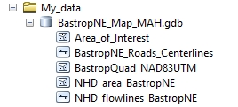
Examine the Bastrop_Map_XXX geodatabase in
ArcCatalog. If the above steps were completed
correctly you will see 5 feature classes within the geodatabase,
as shown below (but missing the contours_5m_LIDAR
feature class).
4.33 Creating a Feature Dataset
and Importing Geology Feature Classes
We will need a Feature Dataset (see the lecture notes) within the geodatabase to
hold files we will create by digitizing.
Why? Without a Feature Dataset, the files we will
create could not share a topology. This is a general
rules... all files that share a topology must be contained
within the same Feature Dataset. For this reason, all
files within a Feature Dataset must have the same spatial
reference and "spatial domain" (more on this below).
-
Right-click on your Bastrop_Map_XXX geodatabase, select
"New", then "Feature Dataset".
-
Name the new Feature Dataset "Geology" and
click the "Next" button to bring up the now
familiar Spatial Reference Properties window.
-
Browse to Projected Coordinate System>UTM>NAD83>NAD83 UTM
Zone 14N.prj and select (make sure the right Projected
Coordinate System is in "Name"), then click "Next".
-
In the next window you are given the chance to specify a
vertical datum. The default is none, which means that
if you have elevation information (e.g. features classes of
the type "PointZ",
"PolylineZ") that were collected with a particular elevation
datum (e.g. often NAVD88 for data collected by most GPS
units) the software will not provide a means for converting
the data to a different vertical datum. The vertical datum for the
Lidar data sets we will later use is NAVD88, so we will specify
the same for this Feature Dataset.
-
The final window sets the "XY tolerance" (minimum distance
between between nodes or vertices before they are considered coincident).
See "About XY Tolerance" in ArcGIS Help. Accept the defaults and click "Finish".
-
As above (step 5 in 4.32), Import
a shapefile, this time from the GeoVectorLayers folder,
into the new Feature Dataset.
-
As these (or any other) new feature classes are imported (or
newly created) in a Feature Dataset they may be (?)
automatically added to the ArcMap Table of Contents.
Remove these so that all that remains in the T.O.C. are the
georeferenced geologic map and Area of Interest
layer.
4.34 Creating
New Feature Classes within the Feature
Dataset
We now need to create empty feature classes within the
Feature Dataset to hold any lines, points and polygons that we will
digitize from the georeferenced geologic map, as well as their attributes.
One strategy for doing so is given below. It is not the only way this could
be done, but is relatively simple and straightforward for this fairly
simple map. A more complicated map with more features
might require a different scheme with additional feature
classes and domains.
Once the feature classes are created, we will "edit" them
to store the map features. Read about the general
process and strategies behind editing by searching ArcGIS
Help for "What is Editing?"
-
In ArcCatalog, right-click on the Geology Feature Dataset, select
"New", then "Feature Class..."
-
We need a feature classes for
geologic lines, i.e. faults and rock unit contacts.
In step 6 above, you imported a shapefile that contains an
incomplete collection of geologic lines for this map, but
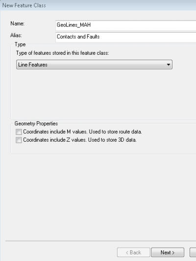
you will also be creating your own. Name this feature class "GeoLines_XXX" (XXX is again
your initials) with an Alias of "Contacts and Faults".
We could separate these into two different line
feature classes but for now faults and contacts will be
stored in a single feature class.
Change the feature "Type" to "Line Feature". The "Geometry Properties" options here should be left
unchecked, as shown below (left).
-
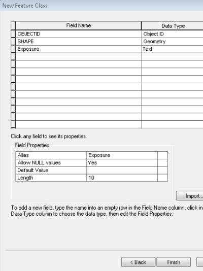
Click the Field Name "SHAPE" to see
the "Field Properties" for the Shape field, (below
right).
-
The "Field Properties" for the "SHAPE" field
of the attribute table for this new Feature Class (which
you've named (GeoLines_XXX) are listed in rows (see
above right). The SHAPE field will
store the "Geometry Type" (in this case lines), coordinates, spatial
reference, and other variables of this feature class. For
more on SHAPE field property variables see pages 45-48 in
the digital book "Building a Geodatabase" or the Help
files.
-
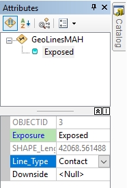
We will now add a few new fields to the attribute
table. Enter the field name "Exposure"
in the blank row below the SHAPE field
name. For future reference, Field Names can not
exceed 13 characters and can't include any special
characters, including spaces. An "Alias"
can be specified for longer names and/or coded field
names. The Data Type for this new field is
"text" (see above right) and the Field Properties list should be
modified as follows:
-
Repeat this process for two new text fields:
-
Field Name: "Line_Type";
Data Type: text, Length: 10 (will eventually
have values of "fault" or "contact") -
Field Name: "Downside"; Data
Type: text, Length:3 (this will have values of N, NE, E, SE, S, SW, W,
NW, or N to indicate the down-thrown side of the fault)
-
Click Finish.
Geologic maps, like the one we are digitizing, contain
many other features besides contacts and faults. For
example, point
features that record attitudes of layering and linear
features and polygons that represent rock units are nearly
always present. We will have the software
create rock units from the lines that we digitize and, in
this instance, you will not digitize the point features.
In a later lab, we will create a features class(es) for
point data (strike & dip or trend plunge of planar or
linear features,
station locations, etc.) but for now just the line feature
class will suffice.
4.35
Adding Domains to the Geodatabase
To avoid entry errors or repeatedly typing the same values
when "populating" the attribute table of the GeoLine_XXX feature class we just created, we will now define lists of
all possible attribute values for the fields we
created, as well as those for a rock unit feature class that
the software will create. Such lists are called
"Domains". Domains are created for the entire geodatabase, not
just for a specific feature class or feature
dataset, allowing the same domains to be used by any feature
class within the geodatabase. Once created and attached
to the feature classes, domain values can be selected during
editing from
drop-down menus in the cells of the attribute tables, a very
fast and efficient way to enter data.
-
In ArcCatalog, right-click the
Bastrop_map_XXX geodatabase icon, select
"Properties..." and click the
"Domains" tab.
-
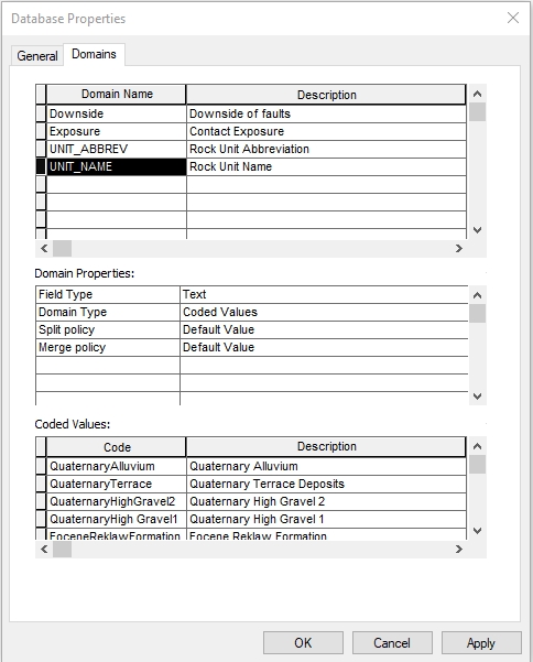
The domains you will create have the following
names, properties and values:
Domain
Name/Description |
Field Type |
Domain Type |
Codes/Descriptions |
| Downside |
Text |
Coded Values |
N, NE, E, SE,
S, SW, W, NW |
| Exposure |
Text |
Coded Values |
Exposed,
Inferred, Covered |
| Line_type |
Text |
Coded Values |
Fault, Contact |
|
UNIT_ABBREV |
Text |
Coded Values |
Qal, Qt,
Qhg2, Qhg1, Er, Ec, EPcb |
| UNIT_NAME |
Text |
Coded Values |
Quaternary
Alluvium, Quaternary Terrace Deposits, Quaternary High
Gravel 2, Quaternary High Gravel 1, Eocene Reklaw
Formation, Eocene Carrizo Formation, Eocene-Paleocene
Calvert Bluff Formation |
All of these domains will be applied to text fields, and all will be
"Coded Value" domains, storing values as codes.
The codes are a way to speed up searching and sorting of the
final tables and have the advantage of providing drop-down
menus for data entry. But using a code different than
the "Description" (the actual value being encoded) produces problems when exporting
the data to other applications (Excel, etc.). I therefore
recommend that the values entered for the Code and the
Description be identical or nearly so, even though this would seemingly
defeat the main purpose of using codes. It's won't
affect searching or sorting for the small tables that we'll
create in this instance, and we won't be
exporting data in any event. Just a word to the wise for
later work. It should also be noted that domain codes
are case sensitive - be consistent and either capitalize (as
above) or don't capitalize the first letter of all of your
coded values.
-
Enter each of the above Domain names into a row below
the "Domain Name" heading. Leave the adjacent
"Description " column blank or type in a description of
what the domain name means.
-
Change the first two rows of the "Domain
Properties" for each domain to "Text" and
"Coded Values", respectively.
-
In the "Coded Values" area, enter the Coded
Values for each domain from the above table, using the
exact same code and description for each value. An
example for the "Unit-name" Domain is shown below. The
"Unit_name" and "Unit_Abbrev" domains will be used for rock
unit polygons that we will later (Lab 5) make with ArcToolbox from the lines we digitize.
Note in the example figure below that the Coded Values have underscores
and/or dashes, not spaces. "Codes" can not contain
special characters or spaces, but "Descriptions" can.
-
Click OK. Other domains and coded
values can be added later, if need be.
4.36
Attaching Domains to Feature Classes
The feature class fields we created earlier do not yet have
their associated domains. It would seem more logical to create
the domains before creating the feature class so that the
domains could be assigned at the same time that the feature classes
were created. This is indeed the recommended
procedure... if you have a well thought-out, preconceived database
schema!
I usually do it the way I'm describing
here...
-
In ArcCatalog, right-click on the GeoLines_XXX feature class in the geodatabase, select "Properties..." and click
the "Fields" tab.
-
Click on the Field Name "Exposure".
-
In the "Field Properties" area, click the blank cell to
the right of the word "Domain" to reveal a
drop-down menu; select the "Exposure" domain.
-
In the blank area to the right of "Default
Value", type "Inferred" (note that these values are
case sensitive and much match the case of the values in your
domains). Dashed lines are by far
the most common type of lines on the geologic map, thus
"Inferred" is a good default value for the
Exposure field.
-
Notice that the software has automatically added a new
field to this feature class: "SHAPE_length",
which will be populated by the software as we draw lines.
-
Repeat steps 2-5, for "Line_type" and
"Downside" using the appropriate domains from
the domain values you earlier entered.
Congratulations, you've now completed the
geodatabase needed for digitizing and creating the map for
this lab!
4.37 Digitizing Features
Some general strategies for digitizing, otherwise known as
"Editing":
- Digitize a map boundary line first (think of this as a
"contact" with the rest of the world).
Alternatively, it can quickly be created from a bounding
polygon automatically, as we will do below, using the
"Feature to Line" tool in the Toolbox.
-
Set Snapping before starting and check and/or reset
Snapping as new feature classes are digitized (more about
Snapping below).
Snapping is ABSOLUTELY ESSENTIAL for results that won't require a lot of further editing.
- Try hard to assure that all line features that intersect
other lines are snapped to those lines or
polygons. Lines can not cross; a vertex must exist
at every line intersection.
- Work from one edge of the map to the other; examine the
map carefully and try to think a few steps ahead.
- Enter attributes as you go. Keep the feature class' attribute
entry window, accessible on the
editing toolbar, open as you work and fill in the fields
after completing each feature.
- SAVE YOUR EDITS OFTEN. SAVING EDITS IS DONE FROM
THE EDITING TOOLBAR, NOT FROM THE ARCMAP FILE MENU.
The editing process can crash the software more easily than
almost any other ArcMap process.
A. Background Info for Digitizing
- General Work Flow For An Editing Session
-
Open ArcMap, add a rectified geologic map image and any
other layers useful for digitizing.
-
Check the Coordinate System of the Data
Frame. Set it to match that of the feature classes you
will edit.
-
If not already open, open the Editor toolbar
(Customize>Toolbars).
-
The generalized digitizing/editing procedure
(for future reference) is:
-
From the Editor toolbar menu (or from a
right-click on the layer of interest in the Table of
Contents), Start
Editing. If the Data Frame coordinate system is different
from that of the editable feature classes in your Table of
Contents, you will see a warning window similar to this:
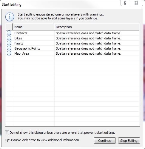
When/if this window appears
and the layer(s) you will edit are listed, "Stop
Editing", go to the Data Frame Properties, and change the
coordinate system to match that of the feature class(es) you
will edit, in this case NAD83 UTM Zone 14N. Although
it may list many layers, the only relevant warnings are for
those you will edit. Ignore any others and hit
"Continue" if the layers you will edit are not listed.
After this warning window, the "Create Features" window
(or Tab) opens, allowing you to select a feature
class to edit and to choose a "Construction Tool" Read about the
"Create Features" window
by searching ArcGIS for "Creating features with feature
templates".
Open the "Snapping Toolbar"
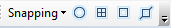 (under the Editor menu on the Editor
Toolbar)
. So what is this snapping business about? (under the Editor menu on the Editor
Toolbar)
. So what is this snapping business about? See "About Snapping"
in ArcGIS 10
Help. READ THIS NOW - IT IS WELL WORTH THE TIME,
CONSIDERING WHAT FOLLOWS.
Begin tracing or outlining a feature – create a “Sketch”. Click to create a vertex; create vertices as needed to
outline the feature. How many vertices and
to what detail do you need to digitize?
This question is best answered by the source layer map
scale. It is senseless to digitize at a scale
greater than 2X the map scale - the map was likely never
intended to have a degree accuracy that exceeds the map
scale, so even 2X is overkill. Finish the feature outline with a double
click, OR a right-click, then "Finish Sketch" OR press F2.
If you don't "Finish" before Saving, you will lose your
edits.
SAVE EDITS (on editing toolbar menu, NOT the ArcMap
toolbar).
Open the table for the newly created feature
(table icon on edit toolbar) and enter attributes.
SAVE EDITS.
Repeat for the next feature.
B. "Digitizing"
the Map Boundary
The map boundary, in this case the Area of
Interest
boundary, is a rock unit contact with the rest of the world
so needs to be stored as a line. Rather than carefully
and tediously tracing the Area of Interest polygon, it
is easier to create an exact replica of the polygon lines using the Toolbox tool "Feature to
Line",
and then to "Append" the result to your GeoLine_XXX
feature class.
-
Use the "Search" tool in the
ArcMap menu to find
the "Feature to Line" Toolbox tool, open it,
"Show Help" and read the Help information
for this tool.
-
Use the tool to create a line
feature class. Change the Input to
Area_of_Interest and accept all of the defaults EXCEPT the
"Output Location", which should be the
Geology feature dataset in your
Bastrop_map_XXX geodatabase. Name the
new line "MapBoundary".
-
Use the "Search" tool again to find
the "Append" (Data Management) tool, open it, "Show Help" and
read the Help information for this tool.
-
Use the tool to append your
new boundary line feature class to your
GeoLines_XXX feature class.
IMPORTANTLY, set the "Schema Type" to "No
Test" (see the tool Help for the reason
why) and accept all other defaults.
-
The GeoLine_XXX
feature class now has a feature stored, but it doesn't have any attributes.
These can be added by editing the attribute
table. "Start Editing", open the GeoLines_XXX attribute table, and click on
one of the empty attribute cells. You
should then see a drop-down menu; choose a
proper value from the list, i.e. these are
"exposed" "contacts".
-
Save your edits and stop
editing.
C. Digitizing Other Geolines
What remains are other rock unit contacts.
Some have been provided(Yahoo!). These need to be
"Appended" to the GeoLines_XXX feature class, then attributed,
following the procedure of Steps 3-6 above.
Append and attribute the the "BastropNEgeolines" feature class to the GeoLines_XXX feature
class by repeating Steps 3-6 above. Exposure is both
"inferred" and "exposed". Check the geologic
map (in the attribute table right-click on the record and
"Zoom to...") for each and attribute accordingly.
There are 76 to do. -
Symbolize the GeoLinesXXX by
Exposure, using a solid line for exposed and a dashed line
for inferred. Pre-made symbols can be found in the
"Geology 24K" Style Reference. Turn it on in the
Symbol Selector and select these symbols - "Contact -
Certain" and "Contact-Inferred" - from the ones available,
or search for them with the Search option.
-
If not already in Editing mode, select "Start
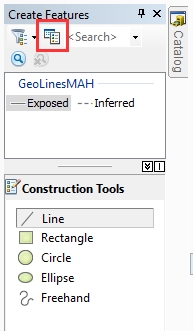
Editing" from the Editor drop-down menu, or right-click on
the GeoLine_XXX feature class in the Table Of Contents and
select "Edit Features>Start Editing". If not already
open, click on the "Create
Features" tab on the right side of the ArcMap window to open
"Create Features" window. With dashed and
solid symbols now assigned to inferred and exposed contacts,
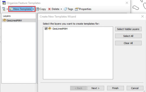
we can create a "Feature Template" for digitizing by using
the button highlighted with the red box, below left. Select
"New Template" (highlighted in red, below right), check on
the GeoLinesXXX layer and click Finish. Henceforth, we
can digitize with the correct Exposure and avoid entering
this attribute in the table each time. Do so now by
selecting either an exposed or inferred line to begin
digitizing (Exposed is selected below).
-
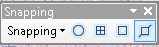
Before beginning, from the Editor toolbar drop-down menu select
"Snapping" to open the Snapping toolbar.
We wish to snap, in this case, to the "edge" of the
Map Boundary lines, not their vertices or ends. Click the
single
icon on the Snapping toolbar that will allow you to do so,
as shown below with the blue-highlighted icon. In
other instances you may want to snap to vertices or ends -
use these options as circumstances dictate.
 Snapping is absolutely
essential when digitizing. Snapping is absolutely
essential when digitizing. Snapping is absolutely
essential when digitizing... It is impossible to
guess when a line you are digitizing is touching
another line unless you snap to it. Gaps between
lines ("undershoots") or "overshoots" can be fixed after a
topology is created, but it is much easier to get it right
the first time! -
Set the map scale to 1:8,000. This is
sufficient detail, keeping in mind that the original map
scale is 1:24000. DO NOT WASTE TIME AT A LARGER SCALE
ADDING MORE VERTICES
THAN ARE WARRANTED OR NECESSARY.
-
Work your way around the map, beginning lines
by snapping to map boundary lines when you can and carefully
tracing lines elsewhere. Double-click to finish, or
right-click and "Finish Sketch", or use the F2 key after
each feature is completed.
-
Remember these rule:
-
Lines should not be
duplicated. They must either start and end
at other lines, or close on themselves to
become "islands", not touching any other
line.
-
Lines must snap to other line edges or vertices and
can not cross. They can abut one another at a
common vertex and continue on, but they can not cross.
-
When a line goes from solid
to dashed, finish the solid line, then
create an inferred line that begins by
snapping to the end of the solid line.
-
Click the Attributes button
 on the Editor toolbar, click a field name (e.g. "Exposure")
and then select the proper domain values from the drop-down
menu. Do not edit the OBJECTID or SHAPE_Length
attributes.
on the Editor toolbar, click a field name (e.g. "Exposure")
and then select the proper domain values from the drop-down
menu. Do not edit the OBJECTID or SHAPE_Length
attributes.
Watch a
short video
of digitizing faults (from a different map). Note that the down-side
attribute is incorrect for some of the faults.
-
SAVE EDITS.
-
Use the pan and zoom tools to navigate the
map, digitizing and attributing contacts as you go.
Topology dictates that
faults and contacts can not cross one another or each
other (geologic reasoning
dictates this too!). The new
contact or fault
should begin by snapping to the start, end or edge of one
that is already
finished.
-
To delete a line
once it's finished, select it (using the selection tool on
the Editor toolbar), right-click and choose Delete
 . .
-
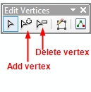
To delete or add a vertex to a completed
line, select the line with the Edit (arrowhead) tool
 on the Editor toolbar, right-click
on the line and choose "Edit vertices" (or select the
"Edit vertices tool from the Editor toolbar, or even
more simply, double-click on the line with the Edit
tool), right-click on the vertex you wish to delete and select "Delete
Vertex"; to add a vertex, right-click on the line
where you want to add one, then select "Insert
Vertex" . Vertices can be moved by dragging
while in the "Edit vertices" mode.
on the Editor toolbar, right-click
on the line and choose "Edit vertices" (or select the
"Edit vertices tool from the Editor toolbar, or even
more simply, double-click on the line with the Edit
tool), right-click on the vertex you wish to delete and select "Delete
Vertex"; to add a vertex, right-click on the line
where you want to add one, then select "Insert
Vertex" . Vertices can be moved by dragging
while in the "Edit vertices" mode.
Yet another way to do this is with the Edit
Vertices toolbar, which is active and on-screen whenever
you are in the "Edit vertices" mode:
-
To split a line into segments, select the
line with the arrowhead tool, find the Split line tool
 on the Editor toolbar and click where you want to split.
-
SAVE EDITS frequently. Once they're
saved, the program can crash and you won't loose any work.
For more on how to create and modify line
features, see "Editing vertices and segments" in the
ArcGIS Help.
-
A final word about
editing... selecting features for editing can be difficult
if more than one layer is selectable - you can
accidentally select a layer that is underneath the one
you're trying to select. To avoid this problem, the
"selectability" of layers can be turned on or off.
The easiest way to do this is by changing the TOC view to
show layer selectability, as discussed in the
last lab. Likewise, when you try to select a layer
and can't, check the Selection TOC view to see if the
layer is turned
off for selection.
Watch a
short video
of digitizing faults and adding/deleting vertices (from a
different map). Note that
the down-side attribute is incorrect for
the first fault digitized.
Watch a
short video
of digitizing contacts (from a different map).
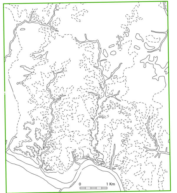
Your completed GeoLines_XXX
feature class should look the image below.
4.38
Create a Topology for the Map
Lines
Before automatically creating rock unit polygons from the
GeoLines_XXX feature class, the
lines must be "cleaned" of errors that will corrupt
polygon creation -polygons will not be created if there are
gaps between bounding lines, and extra
polygons can be created when lines overlap. This is reliably done by
creating a topology layer in the Geology feature dataset that
contains rules designed to spot errors. After setting up
the rules and creating the topology, the topology can be
"validated", and explicit violations of the rules
will be flagged for editing.
-
If you haven't already
done so, Save your edits and
stop editing.
-
From the ArcCatalog window within ArcMap (or from
the ArcCatalog program), right-click on the Geology feature
dataset in your WMA_map_XXX geodatabase, select "New", then
"Topology". The Topology wizard opens.
-
Click "Next", accept the name the new
topology ("Geology_Topology"), and change the cluster
tolerance to 0.1 (0.1 meter; see the description of cluster
tolerance in the Help files).
-
Click "Next" and place a check in
the boxes adjacent to the
"GeoLines_XXX" feature class
- this is the only feature
classes we are checking for dangling and/or overlapping lines.
-
Click "Next" and change the
"Number of Ranks" to 1.
-
Click "Next" to bring up the
Topology Rules dialog. We want to know where contact
lines dangle (not meeting
other contact lines), where they cross other lines
and where they cross
themselves.
a) Click the "Add Rule..." button and select the rule (from the
drop-down menu) "Must Not Overlap".
b) Repeat step a), this time choosing "Must Not
Have Dangles".
c) Repeat step a), this time choosing
"Must Not Self-Intersect".
d) Repeat step a), this time choosing "Must not Self-Overlap"
For a nice explanation of all available topology rules,
search "Geodatabase topology rules and topology error fixes"
in ArcGIS Help.
-
Click "Next" and review a
summary of Topology properties.
-
Click "Finish" and wait for the
Geology_Topology feature class to be created. Answer
"Yes" to Validate the topology now.
-
A new feature class has been created
in the Geology
feature dataset that
highlights every rule violation.
In general, some of
these may be valid exceptions to rules, others
are errors. To see the violations, preview the
topology feature class in ArcCatalog by right-clicking on
the new file, selecting "Item Description" and then the "Preview" tab. The pink squares
and lines are the locations of errors, which we will later view on
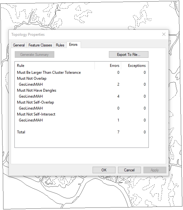
top of contacts feature class in ArcMap. To get a list of errors,
right-click on the topology layer, select
"Properties", click the "Error" tab
and click the "Generate Summary" button.
You can also view the errors
in ArcMap by adding
Geology_Topology to the
ArcMap Table of Contents, as
is shown in the image below.
If you've done a careful job of
digitizing and snapping, your Summary might look something like the one
shown below. The Summary shows 2 errors for the
"Must not overlap" rule, one for "Self
Intersect" and four for Dangles. Yours
could be better (wouldn't that be great!) or
worse (ugh).
End of Digitizing Part 1 (Lab 4)
In Part II of this Lab (Lab 5, next
week) we will go through and
fix the errors before going on to make
rock unit polygons, attribute them, and complete the map.
|
|