Goal

GPS data from last weekend's field trip need to be brought into the GIS project constructed in Labs 5 and 7 and assembled into a geologic map that shows field observations.

Procedure:

The general procedure for lab this week involves the following steps:

1. Import field data into the ArcGIS project created last week;
2. Clean the field data of spurious GPS point and vertices.  Edit your point file attribute table, if necessary, so that joint/foliation strikes and dips are correct;
3. Merge or Append line, point and polygon files to create single feature classes;
4. Edit these lines and polygons to remove any self-overlaps or undershoots;
5. Snap the ends of the line segments to create single lines that entirely enclose areas;
6. Convert the enclosing line features to polygons;
7. For polygons that lie within polygons, subtract the overlying polygon from the underlying polygon -  this step completes polygon creation and editing;
8. Add these new feature classes (the new lines, polygons, and point shapefiles) to your existing GIS from Lab 5 and/or 7;
9. Symbolize the new data to make a map.
10. Hyperlink field photos to locations.

9.1 Getting Started - Importing Field Data

1. Open the Collector App on the iPad, choose "On Device", and "Sync" with ArcGIS Online by touching the cloud icon in the lower right corner of the "WMA_Fall_Final" Map.  Prior to syncing a red dot next to the cloud icon will show the number of unsynced feature edits.  After syncing this red dot will disappear.  This step uploads your field data to ArcOnline.   
   
2. On a desktop computer, open the Lab 7 ArcMap document that you used to create your non-editable Base Layer Feature Layer in ArcOnline. 
   
   
3. Open a Web browser and sign into ArcGIS Online.  Browse to "Content" (a tab at the top), which should list your Web Map, Feature Layers and Service Definitions.  Find your editable Feature Layer and click on its name (e.g. mine last year was called "Mason_WMA_editable_MAH_2017").  This takes you to the "Overview" of this layer.  You should see something resembling the screen capture below.
   
   
   
   
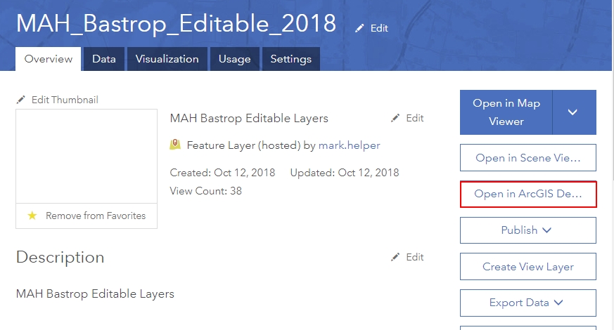
4. Select "Open in ArcGIS for Desktop" from the menu on the right side of the window (shown with red box above).  This will create a downloaded layer (item.pitem) in your browser which you can Save or Open.  "Open" will automatically add the layer to your already open Lab 7 ArcMap document that contains your uneditable base layers after you Sign In to ArcGIS Online again (from ArcGIS Desktop this time) at the prompt.
   
   
5. Your open ArcMap document should now show your editable layers in the ArcMap Table of Contents.  You should be able to see the features you collected in the field on your desktop map!
    
6. Other students are sharing their editable layers too... follow the same steps above to import other's data, following instructions from Nicole.
   
Read on....

9.2 Saving ArcGIS Online Data For Offline Use

The feature layer you downloaded in Step 4 above is not permanently resident as part of your ArcMap document; the feature classes within it are coming from ArcGIS Online and are not stored locally.  The steps below describe a process to create a permanent, offline copy of the feature classes by importing them into a geodatabase. To make the offline copy:

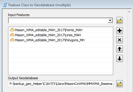
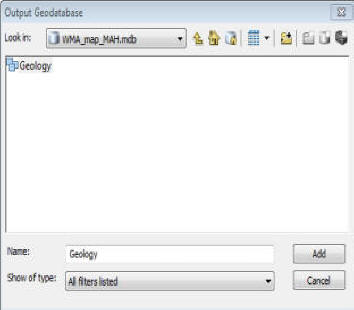
1. Find the tool within Toolbox (from within ArcMap) "Feature Class to Geodatabase (multiple)" and open it.  From the drop down arrow next to 'Import Features" select each of the feature classes (point, line and polygon) THAT WERE BROUGHT IN DURING STEP 4 as the "Import Features".  The "Output Geodatabase" will be the one in your Lab_7_data folder that you created during Lab 7.  When entering the Output Geodatabase, choose the correct geodatabase and select the "Geology" feature dataset as your target. An example using my data from a different project last year is shown below.
   
   
   
   
2. If any of the feature classes within the feature layer failed to import (my attempt with this tool converted the point and line classes but not the polygon class) then in the Table of Contents, use a right-click on the layer (e.g. Polygons_MH), select "Data">"Export Data..." and export the data to the Geodatabase as a feature class (not as a shapefile).  This worked for me when the first attempt failed.  Either or both of these steps adds the newly created offline copies to the Table of Contents (possibly along with other feature class that duplicate what's already there - you can remove these).
   
   
3. Remove the ArcOnline editable layers imported during Step 4 above from your ArcMap.
   
   
4. Import the symbology for your new Point and Line files from layer files in your Lab_7_data folder (Right-click on the layer to be symbolized in the TOC, Properties>Symbology, then use "Import" button and browse to the layer file).  If you didn't make layer files of your symbolized point and line feature classes in Lab 7, then you can simply import them from existing layers in your Table of Contents - i.e. "Point_Data_All_2017" and "Geolines_XXX" using the Properties>Symbology - Import option.  If this doesn't work, then symbolize the three new offline layers the slow way, matching the symbology of existing features, BUT USING A DIFFERENT COLOR AND MAKING THE POINT SYMBOLS A FEW SIZES LARGER SO THESE STAND OUT FROM THE OLDER EXTANT DATA.
   
   
5. Save your ArcMap document with a meaningful name in your Lab 7 or 9 folder.
   
   

9.3 Downloading and Converting Point Data From Avenza Maps

Described below is the technique for downloading Avenza Maps placemarks and attached photos. If you did not collect photos from within Avenza Maps OR the Collector App, my downloaded photos, in a KMZ file in the Lab 9 folder, can be used. If you have photos on your iPad that aren't attached to  locations but you have notes of some kind to indicate location, then download them to a Cloud site (or email them to yourself), carefully rename them according to your notes and skip on to section 9.4.  If you have photos in Avenza Maps, to download:

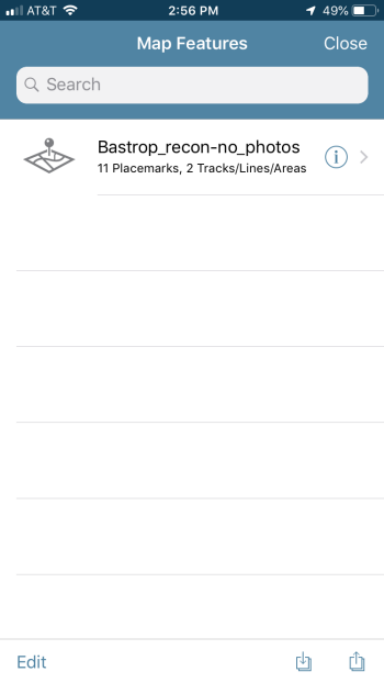
1. With the map containing your points open in Avenza Maps, select the "Map Features" icon, shown below at left in a red square, then choose the "Export" icon at the bottom, shown below at right with the red square.

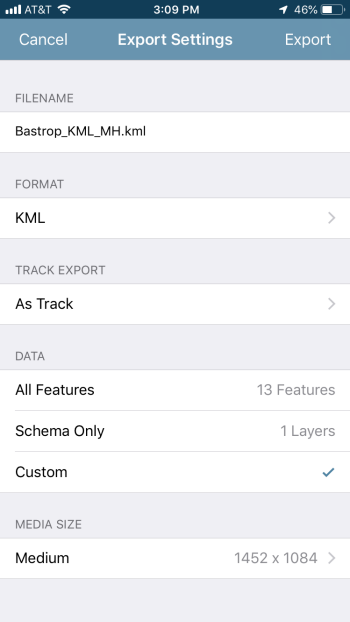
2. In the "Export Settings" window (shown below), enter the File Name "Bastrop_KML_XX" where XX is your initials, choose "KML" as the Format, a destination, either a Cloud storage site (faster) or an Email attachment (slower), and set the "Media" option to export photos if desired.  This will create and export a Keyhole Markup Language (KML) file that can be imported into ArcMap or Google Earth.  With more than one Placemark, Line or Track (and photos, if you choose, at least in the iOS version), a zipped KML file(a "KMZ" file) will be created, which is also readable by both programs.  FYI, GPX and CSV, the other export formats listed, are common exchange format for GPS data, though neither will export photos with the points.  We will not use them, but such files can be imported by many programs and Apps, including ArcMap.  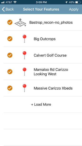Finally, if you choose to, you have some control over which data are exported by selecting from "All Features", "Custom" and "Schema Only" from the Data field.  An example of a "Custom" export with only a layer containing one photo and one track is shown below.  By checking on only the features you want you can control the result, which may be necessary if your field trip features are mingled with those already on the iPad.  Regardless of which options you choose, all data will be exported with GCS WGS84 coordinates, the spatial reference for all KML/KMZ files.
   
3. Within ArcCatalog, create a folder in your Lab_7_data folder named "Bastrop_Avenza Maps_data_XX", where XX is your initials. Retrieve this newly created KMZ file from your Cloud site or email, and copy it to this folder.
   
   
4. Copy your field digital photos from your iPad or phone to the same folder - either email them to yourself (slow) or export to a Cloud site (faster).  Do this even if you exported them within a KML file in the above Step 3.
   
   
5. Use the Search tool in ArcMap to find the ArcToolbox tool "From KML".  The "KML to Layer" tool will convert KML points and/or lines and attributes (but not, unfortunately photos nor, oddly, the "Description" data) to geodatabase feature classes within a newly created geodatabase and adds them to your ArcMap table of contents.
   
   
6. KMZ files can be viewed directly in Google Earth, including attached photos. This provides a means for determining the locations of unattached photos that will later be attached to points. For example, my photos in the Lab 7 folder can be opened from the KMZ file by double-clicking on the icon.
   

9.4 Cleaning Collector App Data By Editing

Field data are rarely perfect; to fix errors we edit.  Polygons collected while streaming may contain spurious vertices that resulted in splitting a polygon into two or more pieces when "submitting" during capture.  Point data may contain invalid strike or dip values, lines may need to be turned into polygons or adjusted in position, etc.  Furthermore, data collected on multiple units needs to be evaluated and duplications removed.  The 50cm resolution orthophoto (available in the lab_7_data >orthophotos folder), added to your map at this stage, may help.  We begin with polygons. Don't forget to turn on or off layers for selection if you have trouble selecting what you want to edit.  You are, of course, familiar with the editing process from Labs 4 and 5.  Below are a few additional pointers and a list of items to complete:

1. To delete a polygon, start editing the appropriate feature class, select the polygon (using any of the selection tools available, including the attribute table) and press the keyboard Del key, or right-click in the polygon and choose "delete".
   
   
2. To edit polygon vertices, start editing, select the polygon, right-click on it and "edit vertices".  Move, delete or insert vertices as needed.
   
   
3. To combine overlapping polygons, select them during an editing session, then use the drop-down menu on the Edit toolbar and "Merge".
   
   
4. To subtract two overlapping polygons, do the same but choose "Clip".  If you use the Clip option, be sure that all base map polygon layers are first turned off in the TOC.  Clipping will clip a hole in any polygon layer beneath the selected polygon (like, for example, the WMA boundary polygon) that is turned on in the TOC.  This procedure only works when both the layer to be clipped (e.g. granite outcrop polygons) and the clipping layer (e.g. grass polygons) are in the same workspace - either in the same geodatabase or the same folder (if shapefiles).
   
   
5. The "Split Polygon" tool on the Editor toolbar can create two polygons from a single one.
   
   
6. To convert closed lines into polygons, first edit them to ensure that the starting and ending nodes of the lines are snapped together, then use the ArcToolbox tool "Feature to Polygon". This tool will fail if the closed lines are not truly closed by snapping.  (This tool also requires that the lines being converted are within the same feature class.)
   
   
7. Once the polygon layer(s) are free of duplicates and error-free, they can be combined into a single feature class, if not already done, using the Merge or Append tool; see the Help files on these tools to learn how.  Add this new layer to the map if not already there.
   
   

It's time for points...

9. Imported point files from Avenza Maps, alas, do not have attribute tables that match our Collector App point layers.  They can nevertheless be Merged together to make a single feature class - do so using the Merge tool.
   
   
10. Edit the attribute table of this merged file to enterstrikes and dips that you might have saved within Avenza Maps; if you did not do so then you can ignore this step.  For future reference, keep in mind that importing KMZ data using the "KML to Layer" tool in ArcGIS does not preserve the "Description" information (such as strikes and dips you may have pecked in...) in Avenza Maps, nor does it import photos attached to points.
     
11. Similarly, enter the PT_TYPE for these same records.  Without this information we can't symbolize the points.
    
    
12. Continue editing... remove duplicate measurements, check that strikes and dips have reasonable values (a strike of zero is probably an error), make sure all points have a PT_type entry (enter one or else delete them).
    
    
13. You will likely find it easiest if the data are symbolized. Use a layer file to do this quickly.  To apply the layer file, open the Symbology tab from the Layer Properties window,  click "Import" and accept the defaults.
     
    
14. Save Edits, Stop Editing.
    

Finally, the lines...

15. Not much to do here, probably only removing duplicates.  See the polygon section for editing instructions.

9.5 Hyperlinking Field Photographs to Field Sites

Read the section "Setting HTML pop-up properties for feature layers" in ArcGIS Help and create HTML pop-up displays for 3 or more field photographs of your choosing.  These will be (or already are if you collected them with Collector) set up as "attachments" on the point feature class (see ArcGIS Help for how to create and enable attachments).  You choose how best to organize the data!  An alternative but less attractive way to do this is to enable the hyperlink tool using a dynamic hyperlink for each point feature.  Search ArcGIS Help for "Using Hyperlinks", paying particular attention to the section on "Defining dynamic hyperlinks though Identify Results".  If you are starting from scratch and want to attach photos not collected as attachments in the Collector App, the preferred method for establishing and viewing hyperlinks is given below.  If you collected points with photos attached, then skip to step 4 below.

1. Rename your (or my photos) photos with meaningful file names so that you can easily know what they show.
   
   
2. We will link photos to the field station points by adding them as "Attachments" to the points.  To add attachments, we first need to "enable" the point feature class so it can contain attachments.  Follow the two steps in ArcGIS Help "Enabling attachments" to do so.
   
   
3. Using the instructions in ArcGIS Help "Adding attachments to feature", attach your photographs to the points where they belong.
   
   
4. Once attached, there are number of ways to view the photos, including using the Identify tool and the attribute table.  Read about these in ArcGIS Help "Viewing attachments".
   
   
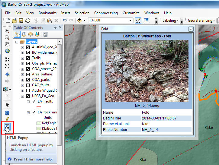
5. Neither of these viewing techniques is very elegant - the picture viewing window often covers the map.  We will instead set up HTML pop-up windows for viewing the photos and attribute information.  Read ArcGIS Help "Setting HTML pop-up properties for feature layers".  We will use the first option mentioned, "As a table of visible fields" that "Include(s) feature class attachments".  Read carefully these sections and create your pop-ups.  It's a lot simpler than it looks and you'll be pleased with the result.  An example is shown below; Popups are launched using the HTML Popup tool on the Main Toolbar, highlighted in red below.
   
   
6. Look at the example below - note the informative title, which was not the default pop-up "Display Expression" (see the Help file on setting up HTML popup properties).  Edit your "comment" field in the attribute table or use an existing comment that describes the photo accurately in lieu of the default display by adjusting fields within "Display" (i.e. changing your "Display Expression") tab of the Layer Properties for the point feature class.
   

9.6 Create a New Map

1. Create a page-size layout of the field trip area over only the region where we collected outcrop data. Symbolize the map to show paleocurrent directions in the Carrizo Sandstone with an arrow symbol (large enough to see!) pointing in the current direction.  Symbolize visited outcrops where photos were acquired differently from those visited where no photos were taken.

2. Summarize your paleocurrent results in a histogram with current azimuth on the x-axis and frequency on the y axis.  Group paleocurrents into 20^o bins - there will be 18 bins on the histogram. Provide this as an inset on the map layout described above.

To Turn In:

The layout described in 9.6 above, AND two screen captures, like that above in section 9.5, that shows a photograph attachment open in ArcMap.

You're Done!

M. Helper, 2007, 2008, 2012, 2014, 2015, 2016, 2017, 2018