|
Messages
Syllabus
Schedule
Lecture
Lab
Projects
Trip(s)
|

 |
Lab 2: Map Projections and Coordinate Systems in ArcGIS v.10
|
|
|
|
|
Note: This exercise is a modification of material
originally developed by Kristina Schneider and Dr. David R. Maidment for CE 394K:
GIS in Water Resources at The University of Texas at
Austin. These materials may be used for study, research
and education. Please credit the authors.
A page of questions from this lab can be found
in the
Lab_2_data folder.
Part 1 - Map Projections and
Coordinate Systems
Contents
2.1 Purpose
- Gain experience in ArcMap using on-the-fly-projection of
various common projections
- Learn how to define a projection in ArcCatalog and
ArcToolbox
- Learn how to project vector data using ArcToolbox
2.2 Introduction and Summary
Recall from lecture that maps are, in essence, graphs and
that creating maps with a computer is analogous to plotting
points and lines on graph paper. For software to show the geographic location of features,
the features must be stored with x and y coordinates tied to a
specific origin (i.e. X=0, Y=0; a "Coordinate System") and
a datum. The datum specifies the dimensions of a model of
the earth; the length of the minor and major
semi-axes of an ellipsoidal earth or the radius of a spheroid (see lecture notes).
Together, the datum and coordinate system comprise the
so-called "Spatial Reference" of a data set.
In ESRI lingo, Spatial References are of two types:
- A Projected Coordinate System ("PCS"), is composed of
a datum (e.g. WGS84) and
coordinate system parameters (e.g. location of origin and
standard parallel(s) in lat. & long., type of developable surface, false
easting and northing, etc.; see lecture notes) specific to a
map projection.
PCS coordinates of features are stored in meters or feet relative
to the PCS origin.
- A Geographic Coordinate System ("GCS"),
includes only a datum, location of a Prime Meridian (Y-axis;
the X-axis is always the equator), and an angular unit of
measure. A GCS has units of decimal degrees - GCS coordinates of features are stored in degrees of latitude and longitude.
West longitudes and South latitudes are stored as negative
values and the units are decimal degrees (DD),
not Degrees,
Minutes and Seconds (DMS).
One of the principal, traditional strengths of GIS software
is the ability to convert data stored in one Spatial Reference
to another Spatial Reference. This map projection
process may involve
conversion of coordinates from one GCS to another GCS, from a GSC to a PCS, or from one PCS to another PCS. A computer
screen or paper map can only have one Spatial Reference; one
origin and one set of axes for the graph.
Thus, the ability to convert coordinates from one Spatial
Reference to another is a key aspect if one wishes to
simultaneously view data sets that have different Spatial
References.
Within ArcGIS, ArcToolbox has tools to do these conversions.
In so doing, you can create a new, permanent data file containing coordinates in the new Spatial Reference. Alternatively, temporary ("on-the-fly")
conversion to a different Spatial Reference is done
automatically upon adding data in ArcMap. This
on-the-fly conversion permits viewing of data sets that have
different Spatial References without first having to create a
new file(s) of converted coordinates with an ArcToolbox tool.
For either of these processes to work the software
must first know the Spatial Reference of the dataset(s). If this information is missing
from a dataset, then ArcToolbox and ArcCatalog have tools for creating
it, a necessary first step (called "Defining a Spatial
Reference" or "Defining a Projection") before
permanent or on-the-fly conversion can be successful. Many older data sets are
missing Spatial Reference information and can produce problems
if this "defining" step is ignored. Worse
still are datasets with the wrong Spatial Reference
definition! We will learn to recognize datasets with
these shortcoming and to apply appropriate fixes.
2.3 Data
Files for this exercise are contained in the Lab_2_data
folder, which resides in the "2017_Labs"
folder. To
use the files, copy the entire Lab_2_data folder to your
network storage space.
Some of the data are within a geodatabase, called Mapproj.mdb, that
contains four feature datasets:
- World: containing feature classes cntry94 and
world30 - countries, and 30º meridians and parallels
for the earth
- USA: containing feature classes States,
Counties and Latlong - states and counties of
the US and a 5º grid of meridians and parallels
- Texas: containing Quad75 and Onedegtx - a
coverage of Texas showing a 1º grid and 7.5' quad map
extents
- Austin: containing Juris, Lakes,
Roads - administrative boundaries of legal
jurisdiction, lakes and roads in Austin, Texas.
All
of these datasets have GCS NAD83 coordinates.
Other data are contained in three shapefiles in the folder
Shapefiles:
- cenart.shp - center lines of arterial streets in
the Austin area
- polylakes.shp - lakes in the Austin area
- creeks.shp - creeks of the Austin area
All of these shapefiles also have GCS NAD83
coordinates, but the latter two are missing Spatial
Reference information.
Finally, there is a color-infrared orthophotograph
of part of Austin contained in a separate folder
called Austin_E_DOQ_SW. This is a Mr. SID format,
1-meter resolution image of the SW quarter of the Austin East
7.5' topographic quadrangle obtained from
TNRIS. The spatial reference for this file is UTM
zone 14, NAD83, but, like two of the shapefiles, this
information is not present in a form that can be read by the
software.
- Copy the Lab_2_data
folder to your network storage space for
this class.
- Create a link to
this folder in ArcCatalog (see
Lab 1
if you've forgotten how).
2.41
Projections of the World
2.410 The
World in Geographic Coordinates
2.411 Loading Data
- Start ArcMap, choosing “New Maps>Blank Map”
and set the default geodatabase for the project to
Mapproj.mdb. Once ArcMap opens, there will be
a single Data Frame called "Layers" in the Table Of Contents
(TOC).
- Right-click on "Layers", and choose Properties. Select
the General tab, and change the Data Frame name to
“Geographic Coordinates”. Click OK.
- Click the Add data button
 , navigate to your
Mapproj.mdb geodatabase and add
all of the World feature dataset feature classes. , navigate to your
Mapproj.mdb geodatabase and add
all of the World feature dataset feature classes.
- If necessary, drag cntry94 above world30 in the TOC.
Watch a
short video
of these steps.
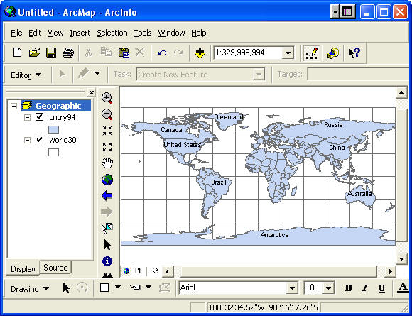
2.412 Symbology and Labeling
You want to make the layer world30 rectangles show
just their outlines, so that if needed you can show meridians
and parallels on top of the countries. You would also like
to label a few of the countries.
- Right-click on the world30 layer in the TOC and
select Properties. Navigate to the Symbology tab and click
on the rectangle in the Symbol cell to get the Symbol
Selector window. Select the Hollow color and press OK. You
should see the world in geographic coordinates.
-
To label just a few features, first right-click on the
cntry94 layer in the TOC and deselect Label Features
(if its on). On the Drawing toolbar (normally at the bottom
of the window), there is a Label button
 that allows you to label individual features. It is found
underneath the big
that allows you to label individual features. It is found
underneath the big
 symbol in the Draw toolbar. If you don’t see the Draw
toolbar, navigate to the "Customize" menu, and click on
Toolbars>Draw to make it visible.
symbol in the Draw toolbar. If you don’t see the Draw
toolbar, navigate to the "Customize" menu, and click on
Toolbars>Draw to make it visible.
- Click on the label button
- Keep the selections chosen by the computer in the
Labeling Options window. Close the Labeling Options window,
and click on the countries on the map that you would like to
label.
Watch a
short video of these steps.
Note: when labeling this way the
program assumes you want to label features in the topmost
layer of the TOC. Be sure to have the cntry94
feature class as the uppermost layer in your TOC or you will
get numbers from the world30 boxes when you click on
the countries to label them.
Where does the label button get the names for the
countries? To answer this question:
- right-click on the
cntry94 in the TOC, select Properties and choose the
Labels tab.
The label tab contains a drop-down menu
called "Label field" that contains all of the field names in
the cntry94 attribute table - it has been set to NAME.
The attribute table for cntry94 contains a field called
"NAME" that contains country names.
- See this for yourself by
opening and examining the attribute table for this layer.
This is
where the label button looks to find the text for the labels
(as do all other automatic labeling tools). Note that from this tab you can
also control the label font, its
placement, the scale at which it is displayed, and select from
some predefined styles.
Watch a
short video
of these steps.
2.413 Coordinate Display
- Move the cursor around on the map and you will see a
pair of numbers at the bottom right that change as you move
the cursor. These give the location of the cursor, and from
the values displayed you can see that these data are
latitude and longitude displayed in decimal degrees.
If you find that the units displayed are described as “Unknown Units”, you can reset “Unknown
Units” to “Degrees Minutes Seconds” (or any
other units) by right-clicking the Data
Frame name in the TOC, clicking the General tab, and changing the
Display drop-down menu to “Degrees Minutes Seconds”.
There are a number of other unit choices, e.g. meters,
kilometers, feet, etc. that can be accessed here too, but
many won't make sense for the spatial reference being
displayed. Remember, these are based on a coordinate
system origin that is specific to the projection. For
unprojected data, it makes no sense to ask for a display of
feet or meters!
- Likewise, you can change from “Degrees Minutes Seconds”
to "Decimal degrees" using the same procedure. Do So.
- Now, SAVE YOUR MAP as World.mxd (mxd extension will
be added automatically).
Watch a
short video
of these steps.
|
|
|
Questions:
1.1.1 What is the spatial extent of the view
shown in degrees of latitude and longitude?
1.1.2 Where is
the point (0,0) (deg. longitude, deg. latitude) located?
1.1.3 Using the Rectangle tool  in the Drawing toolbar, draw a box around
Australia. What is the extent of this box? Give the
coordinates of the lower left corner and upper right corner in
decimal degrees. in the Drawing toolbar, draw a box around
Australia. What is the extent of this box? Give the
coordinates of the lower left corner and upper right corner in
decimal degrees. |
|
|
2.411 The World in Robinson Projection
So far, we have examined the world as “unprojected” data
(i.e. in geographic coordinates). Now we will view the layers
cntry94 and world30 as projected data. A common
projection for the world is the Robinson projection.
2.4111
Creating a new Data Frame and adding data
- Create a new Data Frame, using Insert->Data Frame.
- From the View menu, select Data Frame Properties. Select
the General tab, and name the Data Frame Robinson.
- Right-click on the world30 feature class in the
Geographic Coordinates Data Frame, select Copy, then
right-click on the Robinson data frame and select Paste
Layer. You’ll see the world30 feature class
appear in the Robinson Data Frame.
- Do the same for the cntry94 feature class. Put world30 on top of cntry94 for
visual comparison of meridians and parallels.
- Right-click on the Robinson Data Frame and select
Activate to display the data in this frame.
Without this crucial last step, you will not be able to
do anything with this new Data Frame.
To copy the two feature classes as a group, you
could have:
- right clicked on the original Data Frame in the table of
contents (with Display tab active) and created a new "Group
Layer";
- Dragged and dropped individual layers onto the new Group
Layer;
- Copied and pasted the entire group layer to the new Data
Frame.
This alternative method can be very helpful when dealing
with a large number of layers.
Watch a
short video of these steps.
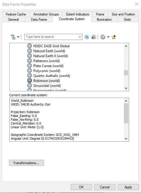
2.4112
Setting the Coordinate System for a Data Frame
ArcMap has the ability to take data that are either
in geographic coordinates or in any number of projected
coordinate systems and project them to a new coordinate system
within the Data Frame ("on-the-fly" projection). To set the coordinate system of
the Data Frame (in this case to the Robinson projection):
- Right click on the new Robinson Data Frame and select
Properties.
- On the Coordinate System tab, under the Select a
Coordinate System box. Then
select Projected Coordinate Systems>World>Robinson
(shown below). Click
OK.
- A warning may appear, but we can ignore it for our
purposes (just click Yes). Ignore this message every time it
appears throughout THIS exercise (in other circumstances you
may need to deal with this issue; we'll cover it in
lecture).
You will see the world map appear in a Robinson projection.
Pretty slick! As you can see, the landmasses appear much less
distorted in this projection. It is important here to note
that the files themselves have not been projected
permanently—they are only displayed in the new projection.
This is called “on-the-fly” projection in ArcMap, which is
distinct from create new data files in different projections,
sometimes referred to as "hard projection", using
ArcToolbox.
- To better distinguish the two views of the world, change
the color for cntry94 in the Robinson Data Frame
Watch a
short video
of these steps.
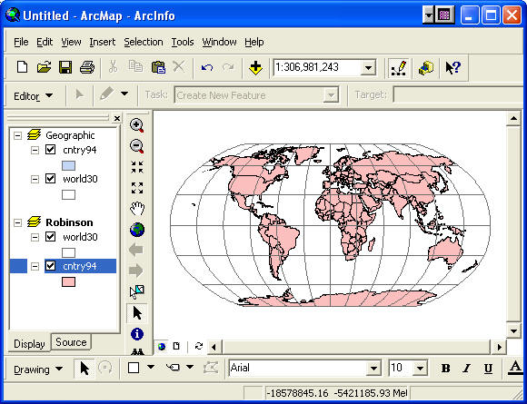
The Robinson projection is a relatively new map
projection for the earth designed to present the whole earth
with a minimum of distortion at any location. If you move the
cursor over this space, you'll see that the coordinates are
now projected coordinates (i.e. eastings and northings)
reported in meters.
2.4113
Create your own Map and layout of several Data Frames
- Create another Data Frame, and copy/paste the layers
from the "Geographic Coordinates" Data Frame into the new data frame. Be sure
to put world30 on top of cntry94 for visual
comparison of meridians and parallels.
- In the new Data Frame, play with the different
projections available in the Coordinate System tab of the
Data Frame Properties, and explore the different shapes the
world can take.
- Note that if you want to view a different Data Frame,
right-click on the Data Frame name, and choose Activate.
- After you’ve experimented with different projections,
select one for a layout you will turn in.
- You can create a layout that contains several different
data frames. Switch to the Layout view, and you’ll see all
three Data Frames displayed. By default, the Data Frames are
on top of each other.
- Resize and reposition these frames to create a more
attractive map layout.
- Be sure to add all the necessary elements to your layout (title, name, date, etc.; a scale bar is not needed for a map of the world!).
Consult the layout guidelines for help. Also, be sure it is clear which
Data Frame corresponds to which projection - give each a caption or
title.
- Save the map file.
|
|
To be turned in: a color layout
showing the world in geographic coordinates, in Robinson
projection, and a projection of your choosing. Before
finalizing your layout, drag the lat-long grids below the
countries to enhance map readability. Title the layout
"Map 1: Projected And Unprojected Maps Of The
World". |
|
|
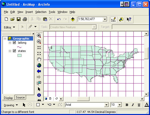
2.42 Projections of the United States
2.421 United States in Geographic
Coordinates
We will now examine map projections used for the
continental United States. We could continue adding Data
Frames to the previous map file, but to simplify things, let’s
create a new map file.
- Use File>New>Blank Map to create a new map file.
- Rename the Data Frame “Geographic Coordinates” and set
Display units to decimal degrees.
- SAVE the map file as USA.mxd.
- Add the states and latlong feature classes
from the USA feature dataset of mapproj.mdb.
- Move states below latlong in the TOC, if
necessary.
- Use the Zoom In tool and zoom to a view of just the
continental US (exclude Alaska and Hawaii). Use the Pan tool
to move the US into the center of the view window if
necessary.
Watch a
short video of these steps.
|
|
Questions:
2.1.1 What is the geographic extent of the
United States? Give the eastern and western limits of
longitude and the northern and southern limits of latitude of
the continental US (not including Alaska or Hawaii) to the
nearest degree.
2.1.2 Which parallel defines much of the
border between the United States and Canada?
2.1.3 If we
removed a wedge out of the earth cut along the meridians
defining the most eastern and western points in the
continental United States, how much of the globe would we have
cut out? Give your answer as a percent of the total volume of
the earth (assume the earth is a sphere for this
problem). |
|
|
2.422 United States in Albers
Equal Area Projection
The Albers Equal Area projection has the property that the
area bounded by any pair of parallels and meridians is exactly
reproduced between those parallels and meridians in the
projected domain. That is, the projection preserves the
correct area of the earth. For example, an island with an area
of 100 km2 will exhibit an area of 100 km2 in the Albers Equal
Area projection. The drawback to this projection is that
it distorts direction, distance and shape somewhat.
- Create a new Data Frame and copy and paste in the layers
latlong and states from the previous frame.
- Make sure states is below latlong to
enhance visual comparison of meridians and parallels.
- Rename the data frame Albers Equal Area.
- Bring up the Data Frame Coordinate System tab. Select
the coordinate system Projected Coordinate
System>Continental>North America>USA Contiguous Albers Equal
Area Conic. Zoom into the continental US.
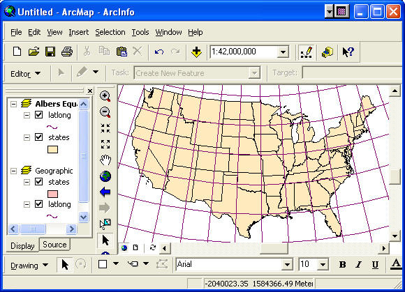
- Compare the United States in geographic coordinates and
in the Albers projection. You should change the color of one
of the layers to further distinguish them.
Watch a
short video of
these steps.
You will see that in geographic coordinates, the United
States appears to be wider and flatter than it does in Albers
Equal-Area Projection. This does not occur because Canada is
sitting on the USA and squishing us! This effect occurs
because as you go northward, the meridians converge toward one
another while the successive parallels remain parallel to one
another. When you reach the North Pole, the meridians converge
at a point. In an unprojected view, the meridians are drawn as
parallel lines instead of converging lines. Drawing the
meridians in this manner distorts the regions between them. As
you approach the poles, the meridians have to be drawn farther
and farther apart in order to make them parallel. For this
reason, distortion of the regions between parallels increases
as you move toward the poles. A more precise geometric
explanation is provided below.
If you take a 5 degree box of latitude and longitude, such
as one of those shown in your ArcMap file, the ratio of the
East-West distance between meridians to the North-South
distance between parallels is Cos (latitude): 1. For
example, at 30°N, Cos(30°) = 0.866, so the ratio is 0.866 : 1,
at 45°N, Cos(45°) = 0.707, so the ratio is 0.707 : 1. In the
projected Albers Equal Area frame the result is that square
boxes of latitude and longitude appear as elongated
quadrilaterals with a bottom edge longer than their top edge.
In geographic coordinates, the effect of the real convergence
of the meridians is lost because the latitude and longitude
grid form a set of perpendicular lines, which is what makes
the United States seem wider and flatter in geographic
coordinates.
|
|
To be turned in: A layout showing the United States
in geographic coordinates and in the Albers Equal Area
projection. Before finalizing your layout, drag the
lat/long grids below the countries to enhance map
legibility. Title the map "Map 2: Projected And Unprojected Maps of the Conterminous United States". |
|
|
2.43
Projections of Texas
Note: A summary and commentary on common Texas projections
can be downloaded
here
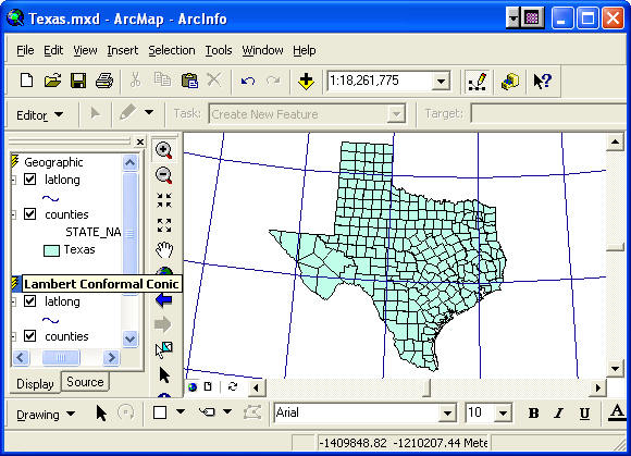
2.431 Texas in geographic coordinates - displaying a
subset
- Create a new map document, Texas.mxd. Name the Data
Frame "Geographic Coordinates".
- Add in the feature classes counties and
latlong (latlong on top) from the USA feature dataset
of the mapproj.mdb geodatabase. The feature class
counties contains counties of the United States,
including Alaska and Hawaii. Make sure latlong is on
top of counties in the table of contents.
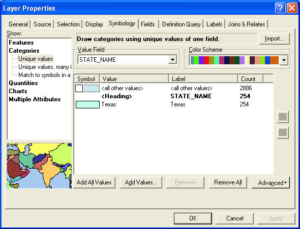
- To make it easier to determine the counties in
Texas, right-click counties, select Properties, and go to
the Symbology tab. Choose to display the counties by
Categories>Unique values, and select STATE_NAME from the
Value Field drop-down menu. Press the Add Values… button
(don't choose Add All Values!), select Texas, and press OK
(you may first have to click the button "Complete List" if
Texas is not displayed in the list). Deselect the check mark
for <all other values>, which will leave only counties
with the STATE_NAME as Texas to be shown. Click OK.
- Only the counties in Texas remain on the map. Zoom
in to see a larger view of Texas counties.
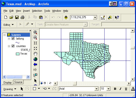
The latitude/longitude grid displayed is in intervals
of 5-degrees. You can determine what latitude or
longitude a particular line represents by moving the cursor to
any line and reading the numbers displayed at the bottom right
below the map view window.
- Save your map document as Texas.mxd.
Watch a
short video of
these steps.
|
|
Questions:
3.1.1 What is the geographic extent of
Texas to the nearest degree in North, South, East and
West?
3.1.2 What meridian runs down the East side of the
Texas Panhandle? (The Panhandle is the northernmost part of
Texas bounded by three lines meeting at right angles.) |
|
|
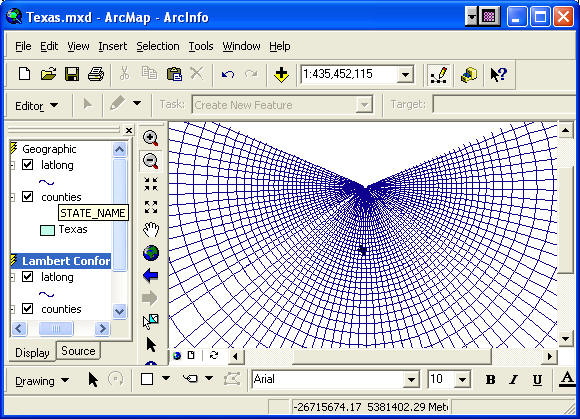
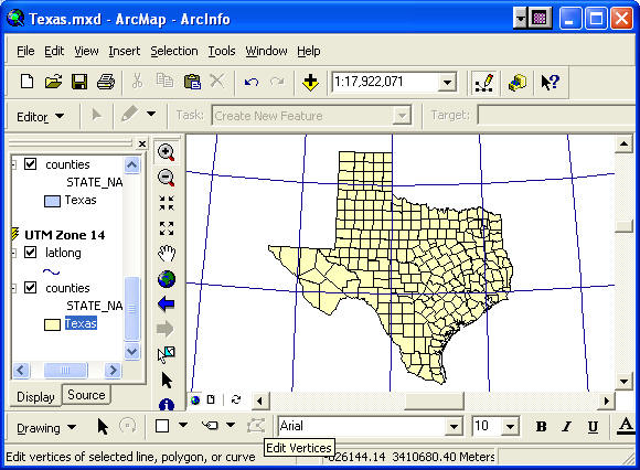
2.432
Texas in Lambert Conformal Conic Projection
The Lambert Conformal Conic projection is a standard
projection for maps of areas whose East-West extent is large
compared with their North-South extent. This projection is
"conformal" in the sense that lines of latitude and longitude,
which are perpendicular to one another on the earth's surface,
are also perpendicular to one another in the projected
domain. Angles remain undistorted in this and all
conformal projections.
- Create a new Data Frame, copy and paste Latlong
and Counties to it from the previous Data Frame. In
the Properties for the new Data Frame, rename the Frame
Lambert Conformal Conic, move to the Coordinate System tab and select
Projected Coordinate
System>Continental>North America>USA Contiguous
Lambert Conformal Conic projection.
- Click OK.
Notice how the meridians now fan out from the north pole (a consequence of using a
conic projection centered on the axis of rotation of the
earth). The display shown is that produced by cutting the cone
and unfolding it so that it lays flat.
- Zoom to Texas in the Lambert Conformal Conic projection.
Watch a
short video of
these steps.
Notice that Texas appears to be slightly tilted to the right. This occurs because the Central Meridian of the
projection is 96ºW, which would appear as a vertical line in
the display if it were shown. Regions to the West of this
meridian (most of Texas) appear tilted to the right while
those to the East appear tilted to the left.
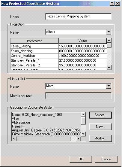
2.433
Texas in the Texas Centric Mapping System - setting a custom
projection
In order to present a pleasing map of Texas, and to
minimize distortion of distance in state-wide maps, the Texas
State GIS Committee has approved a standard projection of
Texas called the Texas Centric Mapping System. There are two variations on this projection, one
is a Lambert Conformal Conic projection, the other is an
Albers Equal Area. We'll use the Albers Equal Area Conic. The definition of this
projection is:
Datum: North American Datum of 1983 (NAD83)
Ellipsoid:
Geodetic Reference System of 1980 (GRS80)
Map units:
meters
Central Meridian: 100°W (-100.0000)
Latitude of
Origin: 31° 15' N (31.25; we will use 18.0 for the exercise
below)
Standard Parallel 1: 27° 30´ N
(27.5000)
Standard Parallel 2: 35° N (35.0000)
False
Easting: 1,500,000
False Northing: 6,000,000
This means that the standard parallels (where the cone
penetrates earth's surface) are located at about 1/6 of
the distance from the top and bottom of the state,
respectively, and that the origin of the coordinate system (at
the intersection of the central meridian and the reference
latitude) is south of Texas in the Gulf of Mexico, to
which the coordinates (x, y) = (1500000, 6000000) meters is
assigned so that the coordinates of all locations in
the state will be positive.
- Create a new Data Frame, and copy/paste Latlong
and Counties to it from either of the previous Data
Frames.
- Double-click on the Data Frame name, select the General
Tab and rename the Data Frame "Texas Centric 35.0".
- Click on
the Coordinate System tab.
- Click on the Add Coordinate System (globe with yellow
asterisks icon), then New, to create a new Projected Coordinate
System. Fill out the parameters with the values given above
and shown in the picture below. Note that the Latitude
of Origin parameter should be 18, and that no commas appear
in the False Easting and Northings.
- You also have to select a Geographic Coordinate System
to specify the datum. Select North American>North
American Datum 1983.
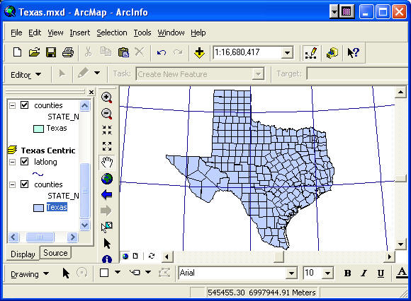
- Click both OKs in the two dialog box and you'll see the
map of Texas transformed to a nice upright appearance, the
Texas Centric Mapping System. Zoom in to Texas.
- Save your work.
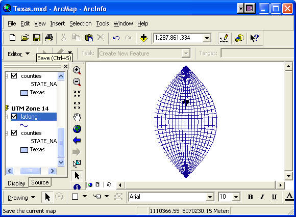
2.434 Texas in Universal Transverse Mercator (UTM)
Projection
The Universal Transverse Mercator projection is actually a
family of projections, each having in common the fact that
they are Transverse Mercator projections produced by wrapping a
horizontal cylinder around the earth. The term transverse
arises from the axis of the cylinder being
perpendicular or transverse to earth's rotation axis. In the Universal Transverse Mercator coordinate system,
the earth is divided into 60 zones, each 6° of longitude in
width, and the Transverse Mercator projection is applied to
each zone.
- As before, create a new Data Frame and copy/paste
Latlong and Counties to it from any of
the previous Frames.
- Double-click on the new Data Frame, and follow previous
steps to rename it UTM Zone 14N. Click on the Coordinate
System tab and select Projected Coordinate
System>Utm>NAD 1983>NAD 1983 UTM Zone 14N
projection.
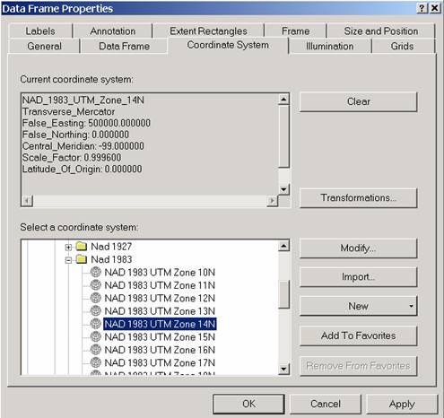
The parameters in the "Current coordinate system" box
mean that the Central Meridian of Zone 14 is at 99°W so that
it covers from 96°W to 102°W; the Reference Latitude is 0.0000
(the equator, which is 0°N); the origin of the coordinate
system is at the intersection of the Central Meridian with the
Reference Latitude and thus is at (0°N, 99°W), where the
coordinates are (x, y) = (500000, 0) m. The False easting of
500,000m ensures that all points in the zone have positive x
coordinates. The y-coordinates are always positive in the
northern hemisphere because 0 is at the equator. In the
southern hemisphere, a false northing of 10,000,000m is
applied to the equator to ensure that the y-coordinate is
always positive.
The Scale Factor of 0.9996 means that along the Central
Meridian, the scale of the map is slightly reduced
(distorted). True (undistorted) scale is only achieved
at two lines of secancy, which are 1.5 degrees to either side
of the central meridian (see lecture notes). The scale
factor 0.9996 describes the maximum distortion within the
zone; scale distortion away from the central meridian is less
than this (more closely approximating a scale factor of 1,
which exists only along lines 1.5 degrees away from the
central meridian).
- Click OK to see the projection applied. The pattern of
meridians and parallels looks very different from those of
the other projections we’ve looked at. Note how the
meridians converge at both the North and South Poles.
Watch a
short video of
these steps. |
|
|
Questions:
3.4.1 How many UTM zones
are there in Texas? Note that the meridians in the
graphic above are not UTM zone boundaries. You may wish
to consult your notes.
3.4.2 Which zone covers West Texas?
Central Texas? East Texas?
3.4.3 In the lab procedure, you
referenced the UTM coordinates for Texas to Zone 14. Why
was this zone chosen instead of the others?
3.4.4. Recall that UTM
zones use a false easting for the central meridian to avoid
negative numbers. Place the cursor over the westernmost tip of
Texas in the UTM Zone 14N data frame, and read the coordinates
from the lower right part of the window. Why is the first
number negative?
- To be turned in: A color layout showing Texas in
Geographic, Lambert Conformal Conic, Texas Centric and UTM
projections. Before finalizing your layout, drag the
latlong grids below the
countries to enhance map
legibility. Be sure to save your map document after you
complete the layout. Title the layout "Map 3:
Projected And Unprojected Maps Of Texas".
|
|
|
2.44
Projections of Austin
2.441 Austin in Geographic Coordinates - Zoom to Layer,
Select by Location, Export to Shapefile
You have viewed the effect of different projections on
different scales. from the world to country and state levels. In
the next few steps, you will take a look at the City of Austin
and the effect of two map projections upon a map of the
city.
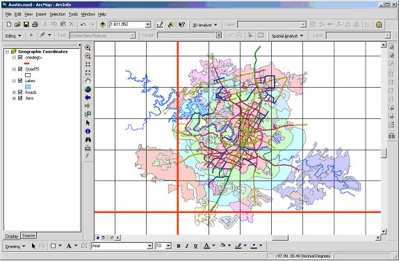
- Create a new map document, Austin.mxd, and add in the
layers Juris, Lakes, Roads from the
Austin feature dataset, and Quad75, and
onedegtx from the Texas feature dataset in the
Mapproj.mdb geodatabase.
The feature class Juris is a coverage of the legal
jurisdictions of the City of Austin. The classes Lakes
and Roads show the lakes and main roads of
the Austin area respectively. The feature class Quad75 is a
mesh of 7.5 minute quadrangles for Texas with map sheet names
for each quad, and onedegtx is a line file of a 1 x 1 degree grid of meridians and parallels. All
of these data are stored in geographic coordinates relative to the
NAD83 datum.
- Double-click on the Data Frame name and rename it
Geographic Coordinates.
- Right-Click on the Juris layer and select Zoom to
Layer.
- Rearrange the layers in the TOC in the following
descending order: onedegtx, Quad75, Lakes,
Roads, Juris.
Make the symbol for Quad75 hollow (See instructions in
Step
1). Symbolize onedegtx using the Highway symbol (Red, size
3). Use a shade of blue for Lakes.
Watch a
short video of these steps.
- You can get a better picture of Austin by using the
Symbology tab for the Roads layer to classify the roads by
size (Size = 1 is the largest road for IH-35 and the Mopac
expressway), and on the Juris layer by Name. The names
correspond to surrounding cities and 2 mile and 5 mile
buffer zones around the Austin city limits, called Extra
Territorial Jurisdictions, or ETJ's.
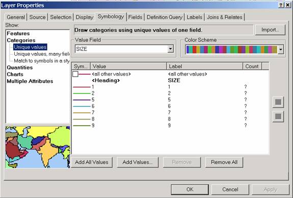
- Right-click on the Roads layer and select Properties,
navigate to Symbology. Select to represent the layer with a
Unique value with SIZE in the Value Field. Use an
appropriate color scheme.
- To make the roads thicker, double-click on the "All
other values" line, to bring up the Symbol Selector window.
Set the Width to 2.00, and then re-click on the Add All Values
button in the Layer Properties window to resize all of the
lines to size 2. Make sure the all other values box is
NOT checked.
- Click OK
- Repeat this process with the Juris layer, placing
Name in the Value field. Change the Color Schemes to
Pastels.
Watch a
short video of these
steps.
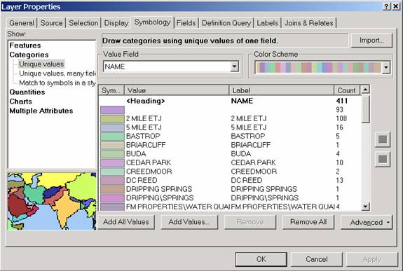
- Click OK. You will see the City of Austin classified by
legal jurisdiction.
- The Quad75 layer shows 7.5 minute quadrangle map
outlines within Texas. Right-click on Quad75 and select
Zoom to Layer so that you see all of Texas displayed in 7.5
min quadrangle sheets.
- Resize the Onedegtx lines to size 1 so that they
are not too dominant in the map. Return to your
previous extent by clicking the blue, left-pointing arrow on
the Tools toolbar.
At this point, we would like to produce a new file that
contains a subset of the 7.5 quad outlines and names for quad maps that cover the Austin area. So far, in order
to focus on particular features in a layer, we have simply
hidden them from display by not including them when we've
symbolized. We would like instead to now extract these
quads from the Quad75 layer and save them as a new
file. The steps are to first select (highlight) the ones
we want, then "export" them to a new file, a shapefile in this
case. To select the 7.5 minute map sheets that encompass
Austin, you will use one of the many selection tools available
in ArcMap.
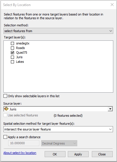
- From the Selection menu at the top of the ArcMap window
choose Selection>Select by Location and fill in the
resulting window as below. This will select features from
Quad75 that intersect (see the Preview graphic at the
bottom of the dialog box that shows polygons that intersect
polygons) Juris.
- Select feature from Quad75 that intersect
Juris.
You'll see a subset of the quadrangles selected on the map after
you click Apply, as shown below (but not labeled).
To export the selection to a new file:
- Right click on Quad75 in the TOC, and select
Data>Export Data... ; ensure that "Selected Features"
appears in the "Export:" drop-down menu and that the "Save
as type:" reads "shapefile".
- Name the resulting file AustinMaps.shp, Browse to the
location where you want to save it (Lab_2_data folder on
your y: drive, perhaps in a new folder), then click OK and
answer yes to add it to the display. Go to
Selection>Clear Selected Features to deselect the quads
you previously selected or simply use the clear selection
tool
 on the Tools toolbar.
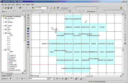
- Delete Quad75 from the TOC.
- Right click on the new
AustinMaps layer in the
TOC and select Label features to show the map names. You can
open the attribute table of this file, called AustinMaps.dbf, in
Excel and copy the list of map names to paste into a Word
document. If you do so, be careful not to overwrite
the original dbf file.
- SAVE your Austin.mxd file.
Watch a
short video of these
steps.
|
|
Questions:
4.1.1 How many 7.5' quadrangle sheets are
there in a 1 degree by 1 degree box?
4.1.2 How many 7.5'
quadrangle sheets are needed to cover Austin? Hint: Open
the Attribute table for the AustinMaps layer and examine the bottom
of the window. The number of records (there is one record for each
quad) in this file is given.
4.1.3 Just
Southwest of Austin there is an intersection of a 1º parallel
and a 1º meridian. What is the latitude and longitude of this
location?
4.1.4 By opening the AustinMaps.dbf in Excel, make a list of
the names of the 1:24,000 scale map sheets (7.5' quads) that are needed to
cover Austin. Cut and paste this list into your answer sheet. |
|
|
2.442 Austin
in State Plane-1927 Projection - Layer Files
The Texas State Plane - 1927 projection is really a family of
projections for Texas, which has five State Plane zones (see lecture notes). Each zone is
projected using the Lambert Conformal Conic projection, with different
projection parameters depending on the zone.
Austin is in the Texas Central Zone. 1927 refers to the
North American Datum (NAD) 27 datum. Unlike 1983 Texas
State Plane projections, 1927 State Plane units are survey
feet (see class notes).
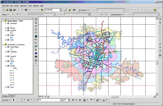
- Create a new Data Frame; name it State Plane – 1927. Add
Juris, Lake, Road, Quad75, and
onedegtx from the geodatabase, as in the previous
Frame. This is easiest by selecting all of the dataset
in the TOC (hold the Ctrl key down as you click on the layer
names), right-click "Copy", click the new Data Frame, and
right-click "Paste layer(s)".
- Click the Coordinate System tab in the frame's
Properties window and select Projected
Coordinate System>State Plane>NAD 1927>NAD 1927 Stateplane Texas Central FIPS 4203 projection. Click OK.
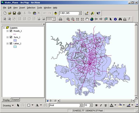
- Right-click on Juris and select "Zoom to Layer".
Play with the Symbology until it looks similar to that in
the Geographic Coordinates Frame. (It may already look
identical - v. 10 seems to have added this feature.
Assume for the sake of the discussion below that the
symbology of the Juris layer in each Data Frame is
different).
Watch a
short video of these
steps.
There are, in fact, two better way to make the
Juris layer symbology match that of the earlier Data
Frame. You could either copy and paste the Juris
layer in from the the previous Data Frame or, to preserve this
symbology for future use, you could create a "Layer
File". A Layer file contains no actual spatial data,
only a description of a layer's symbology. Once created,
it can be applied to the same spatial data in other data
frames or in other map documents. This can be very useful when sharing previously symbolized data with others.
Symbology is only preserved within a map document and is
otherwise not attached to a data file unless it is saved
separately as a layer file. Without a layer file, a
complicated color scheme for a geologic map with many
colors and patterns representing rocks types, for example,
would have to be recreated each time the file was added to a
map document. Thinking back to Lab 1, the reason you
could see the colors and patterns I had created for the
geologic map of Texas was because the map unit polygon file
was accompanied by a layer file.
To create a layer file:
- Activate the Geographic Coordinates Data Frame
(right click, Activate)
- Highlight the Juris layer in the TOC
- Right-click on the Juris title in the TOC, choose "Save
as Layer file...", and save the layer with the default name
to a location on your y: drive.
To apply a layer file's symbology:
- Activate the State Plane Data 1927 Data Frame
- Bring up the Symbology tab for the juris layer
Properties, click the Import button in the upper right,
select "import symbology definition from another layer in
the map or from a layer file" and browse to your saved layer
file before clicking OK.
Watch a
short video of these steps.
|
|
To be turned in: A Layout showing Austin in
geographic coordinates and in State Plane coordinates. Before finalizing
your layout, drag the latlong grid below the
countries to improve map legibility. Title you map
"Map 4: Projected And Unprojected Maps Of Austin,
Texas". |
|
|
2.45
Projection in ArcToolbox
2.451 Project
Wizard
Up until now we have changed the projection of the Data
Frame ("on-the-fly projection") but not the actual projections
of the feature classes. Within the ArcToolbox
module, ArcGIS offers a set of tools to project data files and
save them as a new file in a new coordinate system. There are also a
set of tools for assigning projection information to data that
are already projected, but for which such information is
lacking. This latter process is referred to as
defining a projection or defining a spatial reference, and should not be confused with
the process of actually producing and saving new coordinates for a data
file through projection. We begin first with the
projection tool, "Project Wizard", to project a feature
class.
Before we do, a simple question: If on-the-fly
projection works so well, why bother projecting data to new
coordinate systems? Two reasons: 1) On-the-fly
projections is not as rigorously as actual "hard" projection
of data to new coordinates, so that for exacting work slight
mismatches that result from on-the-fly projection of data in
different coordinate systems are often unacceptable; 2)
Certain geoprocessing tools that compare different data
layers only work if the layers are in the same coordinate
system - one or more layers might have to be converted to a
different projection to use the tool.
- If you have not already done so, SAVE your map document,
always a good practice before using any tools in ArcToolbox.
- Open ArcToolbox from within ArcMap. New in version
10, you do not need to close ArcMap before using ArcToolbox
tools on files that are open in an ArcMap document
if you activate ArcToolbox from within ArcMap.
The same is not true, however, if ArcToolbox is opened from
outside of ArcMap, or sometimes if ArcCatalog is open within
ArcMap. Remember, If a toolbox operation fails, the
first thing you should try is to close ArcCatalog and ArcMap
and try again with stand-alone ArcToolbox.
- Open ArcCatalog from within ArcMap.
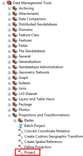
- In ArcToolbox, navigate to
"Projections and Transformations", located in Data
Management Tools. The picture below shows the tools
available for projection in ArcGIS 10.3/ArcInfo (some of
these tools may not be available with an ArcView or ArcEditor
license) that permit projection and projection
definition of "Features" and "Rasters" (more on these data types later in class).
We are going to project the entire contents of the Austin
feature dataset from Geographic coordinates to State Plane
coordinates.
- Expand the Projection and Transformation toolbox by clicking on the + sign
next to it, then double click on "Project" tool.
- Click on the browse folder button in the "Input
Dataset or Feature Class" form field, and navigate to the
Austin feature dataset (notice that we are projecting all
of the feature classes within the dataset in one operation) in
the Mapproj.mdb geodatabase on your Y: drive. The "Input
Dataset..." and "Output Dataset..." fields should now appear
similar to that shown in the picture below.
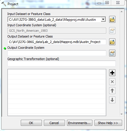
- Press the Select Coordinate System button
 , press the
Select… button. This button will allow you to select a
predefined coordinate system. Navigate through to: Projected
Coordinate System>State Plane>NAD 1983 (US Feet)>NAD
State Plane Texas Central FIPS 4203 (Feet) and click Add,
then click Apply. , press the
Select… button. This button will allow you to select a
predefined coordinate system. Navigate through to: Projected
Coordinate System>State Plane>NAD 1983 (US Feet)>NAD
State Plane Texas Central FIPS 4203 (Feet) and click Add,
then click Apply.
- Press OK. The window now displays the
Output Coordinate System.
- The optional "Geographic
Transformation" field allows us to convert the data to
another datum. Because our new files will use the same
datum (NAD83) as the old files, we do not need to enter
anything here.
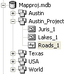
- Press OK. The new feature
classes are created in a new Feature Dataset called
Austin_Project and automatically added to the active Data
Frame in ArcMap.
- Delete these new files from the ArcMap TOC; they are
simply a copy of what you already have, but in a different
coordinate system. They don't look offset from the
other data because they are being projected on-the-fly to
the Coordinate system of the active Data Frame.
Watch a
short video of these
steps.
With just a few clicks, you've projected all of the feature
classes in the Austin feature dataset to State Plane
coordinates!! This process would have taken many more steps
and a lot more time in earlier GIS software. You have
the power! And you’re not afraid to wield it!!
- Within the ArcCatalog tree, browse to the Maproj.mdb geodatabase and you'll
see that you've got a new feature dataset with copies of the
three feature classes in the Austin feature dataset with a
"_1" added to the name of each:
- Open a new ArcMap document.
- Add the contents of the Austin_Project feature
dataset.
- Open the Properties of the Data Frame and change the
name to Projected. Then go to the Coordinate System tab and notice the projection is
NAD_83_StatePlane_Texas_Central_FIPS_4203 (feet), as
required. Pretty cool!!
- Notice the numbers in the lower right hand corner are not
latitude and longitude any more. They are in Texas central
zone State Plane coordinates of feet.
- Right click
Juris, and select Open Attribute Table. Navigate to the
right-hand end of the table. You’ll see that two new fields
have been created, Shape_Length and Shape_Area, which refer to
the length (ft) of the perimeter and the area (ft2) of the polygon, for each
feature in the Juris layer.
Watch a
short video of these
steps.
If you want, you can project the 7.5 quadrangle map and the
1 degree grid similarly and add them to the new data frame.
Verify that it looks the same as the Austin in State Plane
data frame in your earlier map file.
|
|
Question:
5.1.1 The area where the City of Austin has
"Full Purpose" jurisdiction is the area in the center of this
map. The areas around it are areas is where the City has limited
jurisdiction, or that are within surrounding cities. Over what
percent of the area shown in the Juris polygons does the City
of Austin have "Full Purpose" jurisdiction? Briefly
explain how you got the answer, and show any calculations you
use. |
|
|
2.46 Defining a
Spatial Reference
To project data on-the-fly or with a "Project" tool, ArcMap must know the
coordinate system (also called the Spatial Reference)
of the data. Depending on the data type (e.g. shapefile,
feature class, coverage, images; more on this later), this spatial reference
information is either stored internally (geodatabase,
coverage, some rasters) or within a separate
file. When spatial reference information is lacking,
ArcMap cannot successfully project data with different
coordinate systems. This is a common problem for lots of
GIS data, such as shapefiles created with, or for older
versions of, ArcView, many aerial photographs, and
maps you might yourself scan for use in a GIS.
Tools are available in ArcToolbox to create spatial
reference information files. Spatial references can also
be defined in ArcCatalog. ArcToolbox contains
a "Define Projection" tool
for this procedure; in ArcCatalog we can define or alter a
file's XY Coordinate System. Both techniques are examined
below.
2.461 Defining a spatial reference for an
aerial photograph or image in ArcCatalog
- Open a new map document in ArcMap.
- Add the cenart.shp shapefile
from the Shapefiles folder. This file shows
major Austin streets. As before, the Data Frame
adopts the coordinate system of the first file added, in
this case, decimal degrees relative to NAD83 (verify this
by examining the Data Frame Properties).
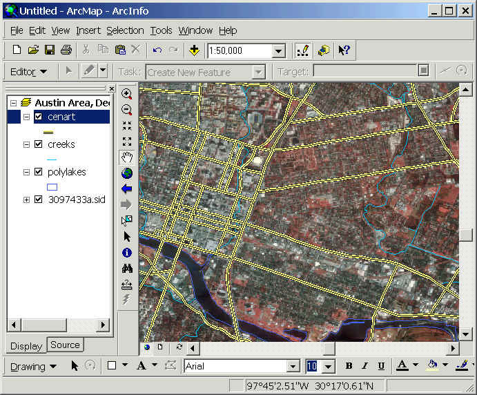
- Click the Add data button and browse to the
Austin_E_DOQ_SW folder of the Lab_2_data folder in your y:
drive and add 3097433a.sid, a digital orthophoto of the SW
quarter of the Austin East quadrangle (which includes the UT
campus). Note that this photo is composed of three
bands; to add all of them at once DO NOT double-click on the
name, rather, click once and then click the Add button in
the dialog box.
- Where is the photo? Even though it was added, it's
not visible in ArcMap. To view it, right-click on the
photo name in the TOC and "Zoom to Layer". Where did
the streets go?
- Note the coordinates in the lower right corner of the
map view window when the cursor moves over the photo - they
are in the range of 100's of thousands and millions of
decimal degrees! Clearly nonsensical. What's
going on?
- Hit the full extent tool on the Tools toolbar. The
map view again goes white - nothing is visible. The
"full extent" of this map covers hundreds of thousands of
degrees in East-West extent and over a million degrees in
North-South extent. The R.F. scale on the menu
bar at the top of the window now reads in the trillions! - the layers are so small at this scale
that they are literally invisible!
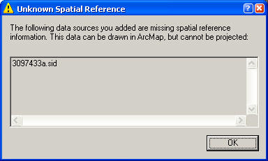
- The problem is that ArcMap has interpreted the
coordinates of the photo as decimal degrees. It has done so
because the photo does not have a spatial reference file,
and the Data Frame coordinates are decimal
degrees. You were warned of this by a message box,
seen below, when
the photo was added. Without spatial referencing
information, ArcMap will always assume that the data are
in the same coordinate system as the Data Frame, in this
case GCS NAD83.
- Close ArcMap, do not save this map document.
Watch a
short video of these
steps.
- From within ArcMap, open Arc Catalog, browse to the 3097433a.sid
file, right-click on the file name and select "Properties"
to bring up the Raster Dataset Properties window shown
below.
- Scroll down in the window to be able to see the "Extent"
and "Spatial Reference" properties, as displayed below.
The Extent defines the area of the air photo (top, left,
right and bottom edges) in coordinates that are clearly not
decimal degrees. What are they? Austin lies at
roughly 3.3 million meters north of the equator; perhaps
they are UTM zone 14 meters. They could equally well
be State Plane Coordinates; it's hard to guess from these
data alone. ArcMap treated
them as if
they were in decimal degrees, thus the problem.
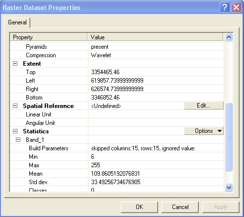
As shown above, the Spatial Reference for this file is
<Undefined> - ArcMap thus had to assume a default, which
it chose as the coordinates of the Data Frame. It's meters, not
decimal degrees, so it chose wrong. To fix the problem
we need to explicitly Define the spatial reference for this
air photo.
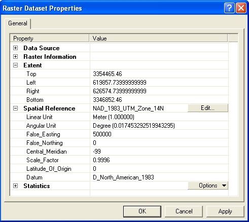
To define the spatial reference:
- In the Raster Dataset Properties dialog box, Click the Edit... button
in the Spatial Reference line, then Select.., then navigate
to Projected Coordinate System>Utm>NAD 1983>NAD
1983 UTM Zone 14N.prj and click Add and OK twice.
- To check your result, examine the dialog box. The spatial reference for the photo is now defined, as shown below.
-
Open a new map document in ArcMap, add the
cenart.shp shapefile first and then add the
3097433a.sid photo. Because you added
cenart.shp first, the Data Frame has an unprojected,
decimal degree coordinate system (the coordinate system of
first file added, remember?).
-
Zoom to the area of the UT campus
and note the close correspondence of the cenart layer with the roads on the photo, like
in the area near the
Erwin Center, below.
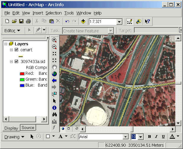
ArcMap has placed the photo, which is stored in
UTM coordinates of meters, on-the-fly, into the decimal degree
coordinate system of the Data Frame! Amazing!
Watch a
short video of these
steps.
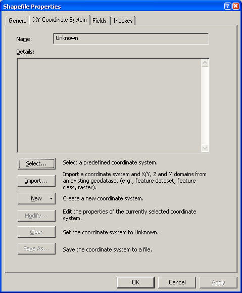
2.462 Defining a spatial reference for a
shapefile in ArcCatalog
-
Within ArcCatalog in ArcMap, browse to your
Lab_2_data Shapefiles folder. Open the folder, right-click
the polylakes.shp file (as the icon and file name
indicate, this is a polygon shapefile of Austin area
lakes) and select Properties... to bring up the dialog
box shown below.
-
As discussed in last week's lab,
this box shows the detailed properties of this file.
If not already on top, click the "XY Coordinate System" tab.
-
This tab gives Spatial Reference of the
file. As shown below, the Spatial Reference is
"unknown", meaning there is no file associated with this
data set that gives the Coordinate System the data are
stored in. As noted above, this is a common
problem for older data sets, particularly shapefiles,
that were created before ArcGIS was introduced in 2001.
If metadata are available this can be corrected.
-
To define the spatial reference in ArcCatalog:
-
Click Select>Geographic Coordinate
Systems>North America>North American Datum 1983.prj,
then Add, then OK.
Through these steps you have created a .prj
file, a file that was originally lacking for this
dataset. The file has the same name as the shapefile,
but with a .prj extension, and is stored in the same
location. ArcMap now has what it needs to properly project this
file on-the-fly.
-
Drag and drop the polylake.shp file from
the ArcCatalog tree into the ArcMap map view.
-
Change the lake symbology to hollow with
blue edges so you can see the photo beneath (drag the lake
layer above the photo in the TOC if it's not already
there).
-
Compare the lake outlines of the photo and
shapefile. They should coincide.
-
SAVE the map document but do not close
ArcMap.
Watch a
short video of
these steps.
|
|
Question:
6.2.1 Give two plausible reasons why the shores of Town Lake on the photo
do not exactly coincide with the Town Lake outline of the shapefile. |
|
|
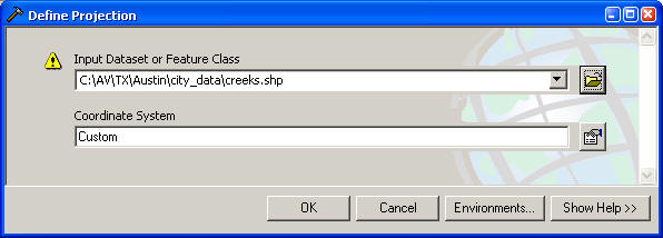
2.463 Defining a spatial reference for a shapefile in
ArcToolbox
A Spatial Reference can also be defined in ArcToolbox.
You might use ArcToolbox for this procedure instead of
ArcCatalog if you had a lot of files to define.
ArcToolbox will allow you to do this in "Batch" mode, permitting definition of a spatial reference for
many files in a single pass. We will do it for just a
single file, which could be done just as easily within ArcCatalog using the
procedure you just completed.
-
The shapefile creeks.shp in the Lab_2_data>Shapefile
folder shows creeks in Travis county. It also lacks
a prj file and thus its coordinate system is "unknown" by
the software. Using the above procedure verify this in ArcCatalog, but DO NOT correct it in ArcCatalog.
-
Open ArcToolbox and find the "Define Projection"
tool by navigating the path: Data Management
Tools>Projections and Transformations. It's at
the bottom of the "Projections and Transformation"
toolbox.
-
Open the Define Projection tool, click the yellow folder button, browse to
your copy of creeks.shp and double-click on the file name
to complete the first step of the wizard, yielding a
dialog box similar to that below (the path to the file
will be different).
-
Press the Select Coordinate System button
,
then press the
Select… button. This button will allow you to select a
predefined coordinate system.
-
Navigate through to: Geographic
Coordinate System>North America>North American Datum 1983.prj,
then click
"Add", "OK", and "OK".
As with the similar procedure in ArcCatalog,
these steps make a .prj file that ArcMap can use to properly
align data during on-the-fly projection.
Watch a
short video of
these steps.
|
|
Question:
6.3.1 You have downloaded digital orthophotographs and several
shapefiles from the web. List the general steps (not
the detailed procedures) that you will do to assure that the data will display properly
(i.e. with the proper coordinates) in ArcMap. |
|
|
You're Done!
|
|
|