7.1 Objectives

This Lab contains 2 parts. In Part A you will:

1. Create a high resolution Digital Elevation Model and hillshade from airborne LiDAR LAS files
2. Create new feature classes in your WMA geodatabase to store field observations;
3. Export your ArcMap project to ArcGIS Online for upload to the Collector App on a field tablet computer;

In Part B, to be done during the following lecture period, you will:

1. Learn procedures for capturing GPS points, lines and polygons with the Collector App;
2. In pairs, practice with a iPad Mini 4 tablet capturing the locations of polygons and lines on the Campus Main Building Mall.

7.2 The Problem and the Data

The goals of our weekend field trip are two-fold:

1. Record the distribution of rock outcrops in the NE corner of the Bastrop Quadrangle.  These cannot be entirely mapped from areal photographs because of masking by vegetation, but are more easily recognized from a "bare earth" Lidar terrain model, which you will create below.  The digital outlines of outcrop polygons allows for a first cut on revisions to the extant geologic map you digitized. 

2. Map and measure the orientation of bedding, joint sets and/or any other planar features in the rocks.  Carrizo Fm.  sandstone has cross beds from which to measure paleocurrent directions - we will record these as well. 

   Data 

The GIS lab portion (Part A) uses the following data:

• UTM zone 14 NAD83, LAS-format, "50cm" resolution airborne LiDAR files acquired in 2017, provided by the Texas Natural Resources Information Service (TNRIS).  These were downloaded from the new TNRIS Lidar data site and unzipped with LASTools.  The NE quarter of the Bastrop Quad is covered by 16 individual tiles that, when unzipped, total 10.7 Gb of data(!). Rather than working with the full quarter quad. we will work with just 6 tiles that cover the south-central portion of the NE quarter, about 4 Gb of data.
  
  
• a UTM zone 14 NAD83, 15cm-resolution, natural color, 2015 digital orthophoto of the NE quarter of the Bastrop Quad. from TNRIS in jp2 format.  This file is about 800 Mb of data. Six inch-resolution(!) data are also available but a bit unwieldy for an area this size.
  
  
• a UTM zone 14 NAD83, ~10 meter-resolution hill-shaded elevation model, stored in ESRI grid format (file name hshade_10m), derived from National Elevation Dataset data, also from TNRIS.  To reduce file size this has been clipped to the boundaries of the the NE quarter of the Bastrop Quad.

**Download the Lab_7_data folder to your flash drive, NOT YOUR NETWORK STORAGE.**  This file contains over 5 Gb of data and may take over 5 minutes to download.

7.3 Working with LiDAR Data in ArcGIS 

LiDAR data are fundamentally clouds of points ("point clouds") with XYZ coordinates and attributes. They are commonly stored and distributed in LAS (LASer) files, a non-propriety format that has gained wide acceptance in recent years.  ArcGIS has extensive tools for importing and working with LAS files.  Our goals for this part of the lab are to:

• Import LAS files into ArcGIS and examine their properties
• Create a raster digital terrain model ("DTM") from these vector files

1. After checking to be sure that the Spatial Analyst and 3D Analyst Extensions are checked on in a blank ArcMap document, open the ArcCatalog window inside of ArcMap, right-click on your Lab_7_data "LIDAR_LAS_files" folder and select "New", create a "LAS Dataset" and rename it Bastrop.lasd.  This creates a container into which we can import LAS files.  A "LAS Dataset" (.lasd) has special properties that allow us to examine some of the unique features of LiDAR data and is required for some LAS processing tools.
   
   
2. Add the six LAS files (each is a tile of a single area and has a file name that ends with .las) to this new LAS Dataset by right-clicking on the LAS Dataset icon, selecting "Properties...", the "LAS Files" tab and the "Add Files..." button (Fig. 3 below).

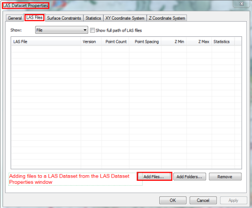
Figure 3. Adding files to a LAS Dataset from the LAS Dataset Properties window

3. Examine the Properties of the imported files. Note that each file contains between 19 to 30 million points - we will be working with over 143 million points in this exercise (!) - that are spaced at about 0.3-0.4 meters (Fig. 4).  The maximum (Z Max) and minimum (Z min) elevation (in meters) of the points in each file are also listed.

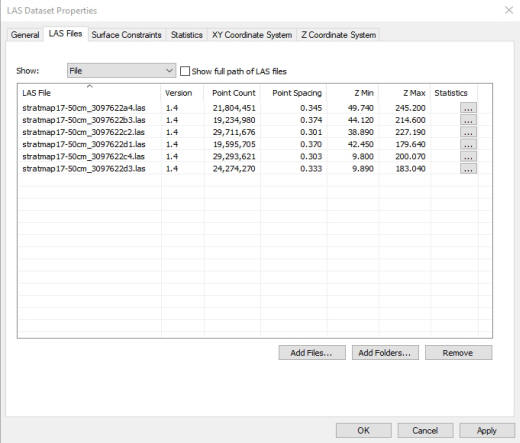
Figure 4. LAS Dataset Properties window, showing point counts, spacings and minimum and maximum elevations for 6 airborne LAS files.

4. Open the "Statistics" tab and click the "Calculate" button - this may take some time... there are over 143 million points(!)
   
   
5. As shown in Figure 5, the result provides Statistics on two important parameters.  This will be important later - pay attention as you read on...

Figure 5. LAS Dataset statistics, summarizing statistics for all six of the LAS files in Figure 4.

LiDAR data consist of multiple "Returns" (upper left table in Figure 5): light pulses that bounce back to the instrument. A "return" is a specific arrival at the instrument from a single laser pulse.  For each pulse, these are classified by whether they return quickest ("First returns") or at successively later times (Second, Third, Forth, etc.).  As shown in the statistic table, of the 143,914,703 returns ("All", the bottom row of the table), about 70% are first returns and 30% are later ("2nd" through "7th" return).  Recently acquired airborne data will also contain a detailed classification of returns based on the origin of the return. Our data are classified into 14 classes (middle table of Figure 5), ranging from Ground (Class 2; these originate directly from the ground) to High Vegetation (Class 5, from tops of tall trees) to Buildings (Class 6) and others.

The distinction between return number (i.e first, second, etc.) and Classification code is important - it is easy to understand that for partially vegetated areas some first returns will come from the ground whereas others will from the tops of trees.  So first returns aren't necessarily what we want for constructing a bare earth model. We are interested in returns that are classified as ground returns - coded 2 or from water - coded 9.  For this dataset, ground returns are only about 55% of all returns and water less than 1%.

The strength or Intensity of returns (middle table) is also measured (on a scale of 0 to 65,535) - some pulses come back strong, some weak.  Strong returns come from highly reflective surfaces, weak from surfaces that absorb or scatter some of the laser pulses.  Minimum and maximum Intensity measurements are listed for each classification.

6. Click "OK" to store the statistics. 

7. Drag the Bastrop.LASD Dataset from ArcCatalog into a blank Arc Map window.  You have just added the entire point cloud, all ~144 million points! 

8. ArcMap shows only the red outlines of each of the six data tiles (this keeps redrawing times reasonable) until you zoom to a specific area.

9. Zoom into the upper left corner (to a scale ~ 1:5,000 or greater) of the lower right tile.  Your screen will look similar to image below.  You are looking at a two dimensional view of a point cloud, color coded by elevation (Figure 6) - the ArcMap Table of Contents shows the range of elevations (in meters) represented by each color.  White represents areas of no data.  These are all of the returned points, regardless of classification or order of return.

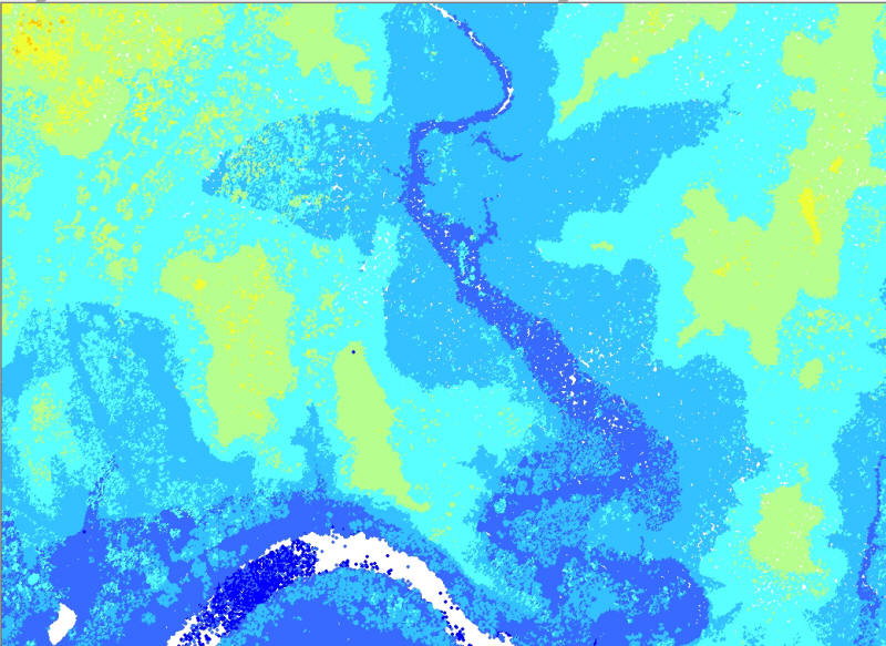
Figure 6. Point cloud data, color coded by elevation.

10. Open the LAS Dataset toolbar (Customize>Toolbars>LAS Dataset), which contains a variety of options for viewing and manipulating point clouds.



If the toolbar is grayed-out, you will have to turn on the Spatial and 3D analysts extensions, as indicated in Step 2 above.

11. Want to see something astounding? Use the Profile Tool (second from right on the LAS Dataset toolbar) to construct a short vertical profile (a cross section) through the point cloud (Figure 7).  A tool tip, visible when hovering the mouse over the tool, explains how.  These are unfiltered points, so we are viewing returns irrespective of Code Classification (tree tops clearly visible!).  We won't spend much time with this tool but it's just too cool to ignore!  Explore the other tools on this toolbar - they provide very powerful ways to view and interactively filter LAS point clouds.  If they don't seem to work, try sampling a smaller area.

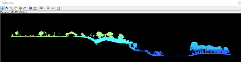
Figure 7. Vertical profile (i.e. cross section) created with the Profile Tool of the LAS Dataset toolbar through a small part of the unfiltered point cloud .  This is a north-south profile across the Colorado River at the apex of the largest meander.  Elevations are color coded and ground vs. vegetation is clearly distinguishable, as is a building and power pole!. 

12. Can't resist one more trick with this toolbar... create a surface elevation model (a TIN; Figure 8) with the Elevation tool on the toolbar by zooming in or out of your Map.

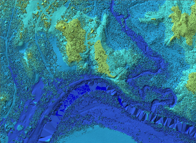
Figure 8. TIN of point cloud data.  The surface roughness is a consequence of vegetation.  The large triangular facets in the Colorado River arise from the lack of points on the water's surface.  They were removed during processing of the raw data to create LAS files so that the river would have a uniform, essentially flat surface.

The maps and profiles created with the LAS Dataset toolbar are visualizations created on-the-fly, not permanent products.  As such, they are of limited use for analysis.  We would like to create a permanent raster dataset from this LiDAR (vector) point cloud - specifically a high resolution, "bare earth" Digital Elevation Model (DEM; nomenclature varies - LiDAR-derived bare earth rasters are commonly referred to instead as Digital Terrain Models (DTMs)).  This will require a tool from ArcToolbox.

13. Using the Search window in ArcMap, search "LAS to Raster" for the tool needed for this conversion.
    


14. IMPORTANT - Before running this tool make sure a) that you are zoomed completely out and can see the red outlines of all of the data tiles in ArcMap; b) that the LAS Dataset Toolbar has the "Filters" tool drop-down set to "Ground" and the Point tool drop-down set to "Elevation", as partially shown below.  These choices will be recognized by the "LAS Dataset to Raster" tool in ArcToolbox if we take care to choose the ArcMap LAS Dataset layer as the Input Dataset and not browse to and choose the original LAS Dataset.

Figure 8a.  The LAS toolbar, showing the Point tool dropdown open and "Elevation" highlighted.

15. Open the "LAS Dataset to Raster" tool from ArcToolbox or the Search window.  If not already shown, show the Help for this tool. You may also need to enlarge the window to see all options, as seen below. USING THE DROP-DROWN ARROW AND NOT THE FOLDER ICON (see Figure 9 below), select Bastrop.lasd as the Input the LAS Dataset.

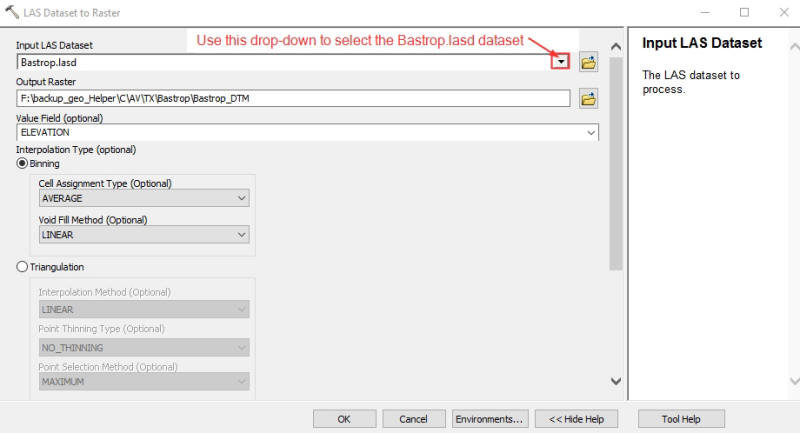
Figure 9.  The LAS Dataset to Raster tool.

• name your output raster BastNE_DTM, to be stored in your Lab_7_data folder
• Value Field is ELEVATION,
• Interpolation Type is Binning with"MINIMUM" (this is a bare earth model...) as the Cell Assignment Type and NATURAL_NEIGHBOR as the Void Fill Method.
• DO NOT CLICK OK YET -we need to specify the raster resolution (cell size), which requires some thought.  The raster cell size should never be smaller than the point spacing of returns.  As seen in the statistics (Fig. 4), the average return spacing is about 0.3 meters. This is for all returns, irrespective of classification.  We are using Class 2 (ground returns) only, not all points, so the spacing for these returns may be significantly greater (3x to 4x greater- not all points will have ground returns).  A conservative approach for a bare earth DTM is to set the raster cell size to ~ 3 times the average return spacing.  This means our bare earth DTM should have a cell size of about 1 meter. So, SET THE "Sampling Value" TO 1.
• Z Factor is 1. Click OK. This will take a few minutes...

If all went well your DTM should look like the Figure 10 below.

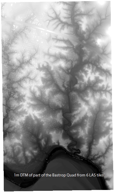
Figure 10. 1m resolution Digital Terrain Model (DTM) created from six LAS files using the LAS Dataset to Raster tool.  Yours should look slightly different, this one is not a bare earth model.

This new DTM will be easier to visualize in shaded relief.

16. Using the Search window, find the Hillshade tool in the Spatial Analyst ArcToolbox and create a Hillshade.  Your Hillshade should resemble Figure 11 below.  Take some time to explore this at higher magnification - it's an amazing product!
    Note:  If the tool gives an error, do use the default file storage locations but instead save it to a flash drive!  Likewise, if the source DTM file is located in network storage, try copying (in ArcCatalog) to a flash drive and use that source DTM instead.
    
    
17. Load the hshade_10 file into your ArcMap project.  hshade_10 is a ~10m resolution hillshade created from a National Elevation Dataset (NED; recall the lecture on Elevation Models) 10m DEM.  NED data are not derived from Lidar measurements.  As illustrated in the comparison below (Fig. 12) and from your own observations, the difference is dramatic.  Fracture patterns that are, at best, obscure in the ~10m data are clearly visible is the 2m DTM.

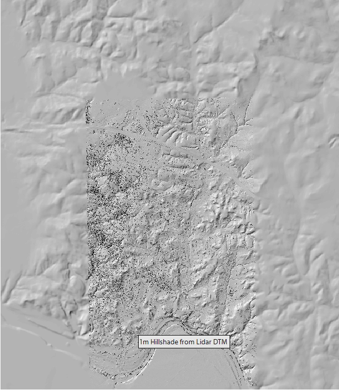
Figure 11.  Hillshade of the Lidar DTM (central region) on top of 10m NED DEM.  Note that this is not a bare-earth model so may look different from yours.

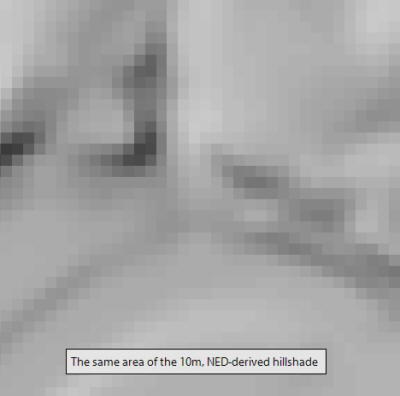
Figure 12.  Comparison of 1m, LIDAR-derived  hillshade and a more conventional 10m, NED-derived hillshade over precisely the same area.  Note the dramatic difference in detail.  The LIDAR DTM is not a bare earth model - buildings and vegetation are clearly visible.

The 1m DTM hillshade is a ~62 Mb file stored in uncompressed ESRI grid format.  We would like a smaller compressed file for our handheld field units.  We can make one by converting the result to a JPEG image.  To do so:

18.  To compress this new raster:

1. Right click on the hillshade layer in the ArcMap table of contents, select "Data">"Export data..." to show the following Export Raster window:



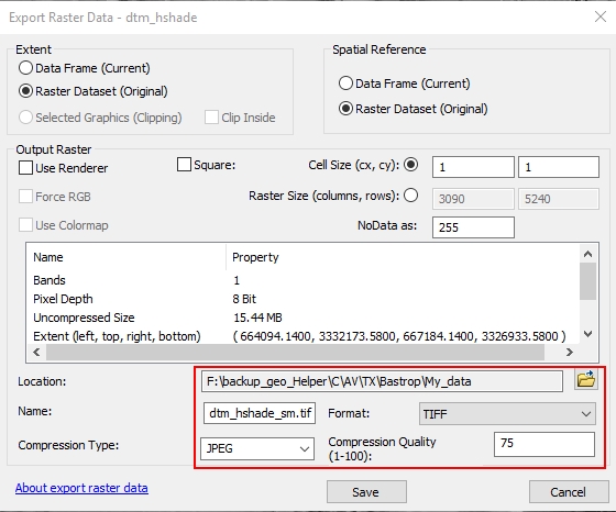
Fill in the fields with the values shown in the red box above, making sure you save this to a place where it can be easily retrieved, and click "Save".  This will create a 1m resolution, JPEG compressed raster, saved in Geotiff format.  Through these processes, we have reduced the file size from ~62 Mb to about 15 Mb without appreciably affecting the utility of the hillshade!  This new Tiff file is now small enough to store and quickly render on our field tablets, but it only covers a small portion of the area of interest.  A ~42 Mb 1m hillshade of the entire NE quarter of the Bastrop Quad, prepared the same way, is in the "LIDAR_hillshade_all" folder of the Lab_7_data folder.  We will use this instead.

7.4 Constructing a Map for Field Work

The field data we will collect includes the outline of outcrops (polygons), joint measurements (point features), bedding and cross-bedding orientations (point features) and photos (tied to points). You digitized a geologic map Lab 4 and 5 that will provide context for your field work.  The LiDAR hillshade created above will do the same. What remains is to create new feature classes within the feature dataset (Geology) of the geodatabase (Bastrop_Map_XXX) you created in Lab 4 that will store your field data. You have already done many of the steps below in Lab 4. Refer to it if you've forgotten how to create feature classes and domains.

1. Open ArcCatalog and browse to the Geology feature dataset of your Bastrop_Map_XXX geodatabase in your Lab_4_and_5_data>My_data folder.
    
2. Time to create the empty Feature Classes that will contain the GPS-derived points and areas...

1. Right-click on the Geology Feature Dataset icon, select "New...", then create new Polygon, Line and Point Feature Classes (named Polygon_XXX, Line_XXX and Point_XXX, where XXX is your initials). Click "Next" and move on to step b below;

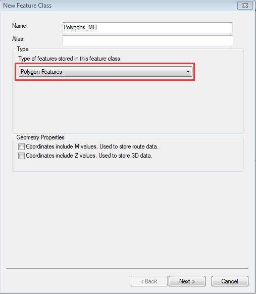
Figure 13. The window for creating a new polygon feature class.
 

2. The polygon feature class will store GPS-derived outlines of outcrops and any other features that are polygons.  We need an attribute field that records the unit being mapped (e.g. Carrizo, Calvert Bluff, etc., or “other”) that can be entered as we collect the data.  So... add two Text fields to the polygon feature class, one called "UNIT" and another called "COMMENT". See section 4.34 in Lab 4 if you've forgotten how. The length of the UNIT field should be 5 and the COMMENT field 30.  Please use these precise field names, including capitalization, for this and all other feature classes. Merging and appending files from different field units is much easier if everyone uses exactly the same field names and properties.
   
   
3. Attach the domain "UNIT_ABBREV" to the polygon attribute field UNIT (again see Lab 4). Finish by clicking OK.
   


4. Repeat Step 2a above to create a line feature class called "Lines_XXX", being sure to change the "Type" to line.
   


5. The line feature class will be used for outcrop outlines that can't immediately be seen to close on themselves (i.e. can’t be mapped as polygons) and other linear features we care to map. The attributes (with Domains) and the new fields to create are:
   
   
   1. 5-character text field, called  "UNIT", that will contain coded values from the Domain "UNIT_ABBREV" (just like for polygons).
     Attach the domain to the field, as above.
   
   2. 10-character text field, called "EXPOSURE", that will contain coded values for the Domain "Exposure". Attach the domain to the field, as above.
      
   
   
   3. 30 character text field, called "COMMENT", without an attached domain.
      
   
   
   4. 3 character text field called "AUTHOR", with no domain but a default set to your initials.
      
   
   
   5. Click OK to finish.
      
      
   6. Repeat Step 2a again to create a point feature class, being sure to change the "Type" to point.
      
   
   
   7. The point feature class will be used to record features too small to be polygons, for strike &dip or trend&plunge measurements and for photographs. We will need fields for:
      
      
      1. 10-character text field, called "PT_TYPE", that will contain coded values from a text Domain called "PT_TYPE" of "Joint", "Foliation", "Bedding", "XBedding", and "Other". Create this new Domain and attach it the PT_TYPE field.
         
         
      2. 5-character text field, called  "UNIT", that will contain coded values from the Domain "UNIT_ABBREV" (just like for polygons).
        Attach the domain to the field, as above.
      
      
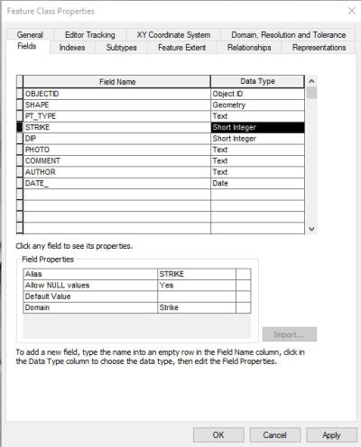
      3. 3-character short integer field, called "STRIKE", that will contain a short integer from a Coded Value Domain called "strike" of every second integer between 2 and 360 (i.e. Codes of 2, 4, 6, etc. with Descriptions of 002, 004, 006, etc., yes all 180 Codes!). Create this new Domain and attach it to the STRIKE field.
         
      
      
      4. 2-character short integer field, called "DIP", that will contain a short integer from a Coded Value Domain called “dip” of every second integer between 2 and 90 (i.e. Codes of 2, 4, 6, etc., with Descriptions of 02, 04, 06 etc.; 44 values in all). Create this new Domain and attach it to the DIP field.
         
      
      
      5. 5 character text field called "PHOTO", with an attached coded value domain call TrueFalse with coded values and Descriptions of "True" and "False".  Create this new Domain and attach it to the PHOTO field.
         
      
      
      6. 30-character text field, called "COMMENT", without an attached domain.
         
      
      
      7. 3 character text field called "AUTHOR", with no domain but a default set to your initials.
         
         
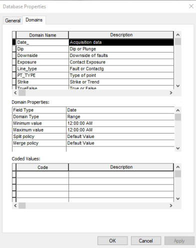
      8. A Date field called "DATE_".  No length or domain is required.
         
         
   8. Create these new Fields and their Domains with the above coded values and attach the Domains to the Fields.  An example of the completed Point Feature Class fields and the new Domains is shown below.
      
      
   9. Test that these new feature classes, when edited in ArcMap, have properly attached domains.  To do so, add the new feature classes to the ArcMap document, edit each in turn, making sure that attributes can be added from drop-down menus.  Do not save your edits, simply test that you can add a point, line and polygon and that attributes can be entered as expected for those that have domains.  IF NOT - make new features classes, reattach the domains, and test again.

What about the raster files?  The Lab_7_data folder contains high resolution DOQs and our newly created Lidar 1m hillshade raster; should we import these into the geodatabase? In this case the disadvantages of doing so outweigh any advantage. In particular, the color DOQ is a large jp2 format file that would get much larger when uncompressed and stored in IMG format, which is the format required by the geodatabase. There is no real advantage to doing this, other than having everything in a single container, and we are left with a file that is >150 Mb. We could instead create a geodatabase raster index (see Help files on this topic), but for the few rasters we will work with this also provides no real advantage. We will keep the rasters separate from the geodatabase for these reasons.

Congratulations, you have now completed the database you will need for this project.

OPTIONAL 7.5 Making a Layout for the Avenza Maps App - Creating a GeoPDF OPTIONAL

1. Open your completed ArcMap from Lab 4&5.  Go to the Layout View and add the Lidar hillshade provided in the Lab_7_dat folder (Lidar_hshade_all) for the entire NE quarter of the Bastrop Quad.  
   
   
2. Load your empty polygon_XXX, line_XXX and point_XXX feature classes you just created and move them to the top of the Table of Contents if not already there.
   
   
3. Order the remaining layers so that the Hillshade is at the bottom, the DOQ is second from the bottom, and all remaining layers above these.
   
   
4. Set the Display Properties of the rock units  to 50% transparent.
   
   
5. Zoom to the Bastrop NE quad. boundary layer and SAVE THE MAP document with a new name to your Lab_7_Data folder, indicating in the file name this is for AvenzaMaps.
   
   
6. Switch to Layout mode.  Go to "Page and Print Setup", uncheck "use printer paper settings" and Set Page to Width: 10.5" and Height to 12".  Got to layout mode, set the map scale to 1:24000 and adjust the edge of the Bastrop NE map to the edge of the data frame to fill as much as possible to the layout boundaries.  We will make one map for display in the  Avenza Map App on the iPads.  This will show the LiDAR hillshade layer turned on with other layers partially transparent above it. Once the layout is satisfactory, go to File>Export Map>, Save as Type PDF, resolution 300 dpi, Image quality Best, Advanced tab> check on "Export Map Georeferencing Information".  This will create a GeoPDF that can be used in the field with your GPS-enabled IPad.
   
   
7. IMPORTANT: IF YOU ARE USING PATTERNS WITH COLORS FOR ROCK UNITS, REMOVE THE PATTERNS FROM THE SYMBOLOGY NOW.  Collector App will not accept polygons symbology that uses patterns.  If you would like to use them again, make a layer file of this layer ("Save As Layer File...") before deleting them.

To get this PDF onto your iPad or other mobile device, it needs to be imported through the Avenza Maps App.  To do so requires that the GeoPDF is in a DropBox, UTBox, ICloud or any other cloud storage space that can be accessed from our IPads or your phone.  If you don't already have one, create a free DropBox Account, being sure to keep track of your user name and password!  Place your GeoPDF in a DropBox folder so it can be retrieved by your iOS (or Android) mobile device.  If you plan on using your smart phone in the field install the Avenza Maps App and load your GeoPDF into it from the App.

7.6 iPad Mini 4 and the Collector App

We will collect field data with iPad Mini 4 tablets running the ESRI Collector App. The iPad Mini 4s as configured are strictly WiFi devices that do not have cellular phone service, though they are capable of such.  With this capability, even when not enabled, they have a GPS that can be accessed by Apps like Collector and Avenza Maps, even when WiFi is not available. FYI, iPads without a cell service capability do not have a working GPS when offline.  To get our desktop GIS onto to an iPad Mini we will first upload "Feature Layers" to ArcGIS Online, then create a map from these layers that can be brought into the Collector App on the iPad Mini.

 REQUIRED 7.6a Uploading Data to ArcGIS Online REQUIRED

In order to use the map data you’ve just created for the field trip, they need to be exported to ArcGIS Online as a service. This will be done three times – once for the features that will be edited in the field (point, line, and polygon), once for features that should not be edited in the field (contours, boundaries, etc.) and once for the LiDAR hillshade raster.

1. Load the Point, Line, and Polygon feature classes that you created in 7.4 and the Area of Interest from Lab 4&5 into a new, empty ArcMap document.
   
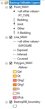
2. Symbolize the point, line and polygon layers to look something like what is shown below.  Note that I've increased the symbol size of all of the point symbols and included red outlines for all of the polygons.  Save your ArcMap document with a name like "Editable Layers" ArcOnline".
   
   
   
3. Click "File > Sign In" and enter your ArcGIS Online Username and Password you created earlier (note that these sign-in credentials are different from the ESRI account you may have created when activating your student trial of ArcGIS for desktop).
   
   
4. Next, click File > Share As > Service. You should see the following (Figure 14):

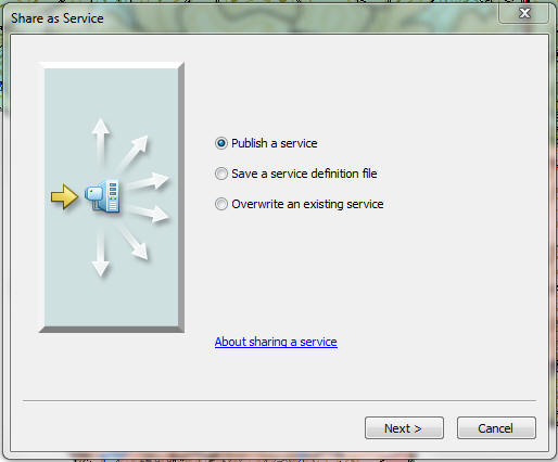
Figure 14.  Share as Service window in ArcGIS Online.

4. Select "Publish a service" and click Next (Figure 15).
   
   
5. On the next screen, click the drop down arrow under "Choose a connection", then select "My Hosted Services". (Your hosted service will be  the University of Texas at Austin).
   
   
6. Choose a descriptive name for the service that reflects the contents of the layers you are exporting.

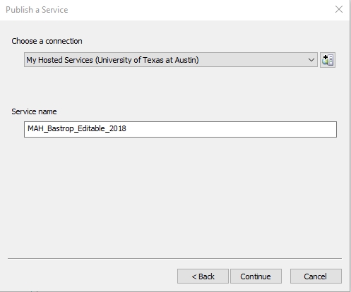
Figure 15.  The Publish a Service window in ArcGIS Online.

7. Click "Continue" to bring up the Service Editor window (Figure 16). The parameters window is grayed out until you change the default capabilities for the service.
   
   
8. In the left panel, click "Capabilities", then check the box for Feature Access and uncheck the box for Tiled Mapping.

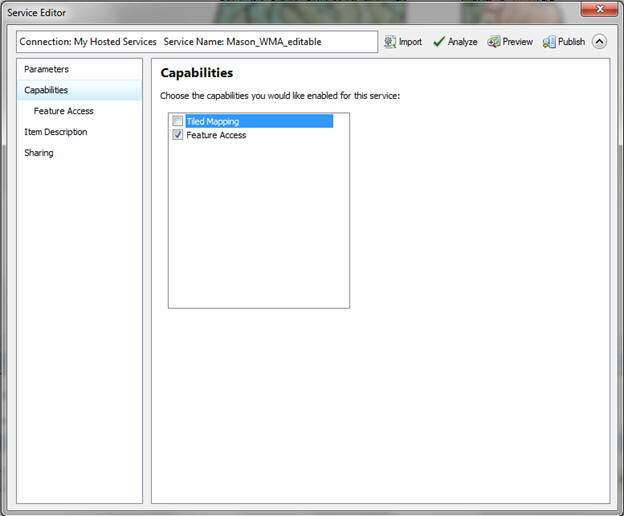
Figure 16.  The Service Editor window in ArcGIS online.

9. Click the "Feature Access" option that is now visible beneath Capabilities in the left panel. If you are publishing a service for your EDITABLE LAYERS ONLY, under Operations allowed, check all of the boxes. This will permit the point, line, and polygon feature classes to be queried, synced, updated, etc. once you are working with these in the Collector App. If you are publishing a service for your NON-EDITABLE features (contours, boundaries, etc.) only check the Query, Update, and Sync boxes.
       The following link includes a description of what each of the configuring options do for Feature Access:
   

   http://server.arcgis.com/en/server/latest/publish-services/windows/editor-permissions-for-feature-services.htm
   

10. Click "Item Description" on the left panel. Fill in the required Summary, Tags, and Description boxes with the requested information.
    
    
11. Under "Sharing" on the left panel, click to enable sharing with the name of your organization (University of Texas at Austin), and, if available, Members of the Group "Geo327/386G Fall 2018 Field Trip".
    
    
12. At the top of the Service Editor window, click the "Analyze" button. You should see a window appear that shows the number of Errors, Warnings, and Messages for your service. Errors will prevent a service from publishing to ArcGIS Online and need to be fixed before publishing.

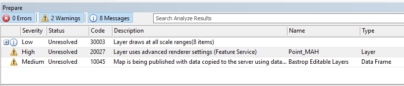
Figure 17.  The results of the "Analyze" request, as shown in the Prepare window of ArcGIS Online, showing Errors (0), Warnings (2) and Messages (8, but collapsed).

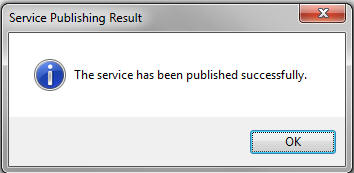
13. Once any errors have been resolved, click "Publish" in the Service Editor window. Publishing can take a few minutes, but if all goes well, you should eventually see the following message:

The steps are identical for the next two services that need to be published (i.e. non-editable features and Lidar hillshade) with a few exceptions. First, the non-editable features.

14. Save and close the ArcMap Editable layers document. Open the ArcMap document that contains your geologic map created for Labs 4&5.  Change any rock unit symbols that contain patterns to simple solid color fills and set the rock unit transparency to 50%.  Go to Layout mode and make sure that your map is centered and entirely visible within the Layout Frame.  If you use the the page size and map scale suggested in 7.5 above this is simple.  Repeat steps 4-8 above.
    
    
15. At item 9 above, only the Query, Update, and Sync boxes should be checked. We do not want to create, delete, or otherwise modify these features.  Repeat items 10-13.  My map took about 5 minutes to "Publish".
    
    
16. For the Lidar Hillshade:
    
    
    1.  Close your ArcMap document and open an empty new one. Load the LIDAR hillshade layer "Lidar_hshade_all.tif". Change the symbology to "Stretched" with a Stretch "Type" of  "None".  Repeat steps 4-7 above.
       
       
    2. Leave the Tiled Mapping Capability checked and do not check Feature Access at step 8.
       
       
    3.  Click "Caching" in the left panel. Caching creates image tiles (see the lecture on rasters) at specified resolutions that will rapidly render on screen when zooming in and out.  The challenge here is determining an appropriate tiling scheme and level of detail that allows us to take advantage of the resolution of the Lidar hillshade without wasting unnecessary space on the ArcGIS Online server. Click the box next to Tiling Scheme, and change the method to "Suggest". Type "5" in the scale levels dialog that opens, then OK.  The options selected below (Figure 18) should be adequate for our purposes and will result in a file that is about 45 Mb in size.  Before leaving Caching, open the "Advanced Setting" in the left menu and set the Tile Format to "Mixed" and Compression to 100.
       
       
    4. Repeat items 10-13.  My hillshade took about 1 minute to Publish and another couple of minutes to create the cache tiles.

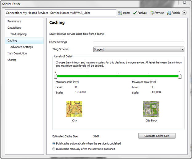
Figure 18. The Service Editor window in ArcGIS Online, showing options for caching a raster, in this case our Lidar hillshade.

When publishing the service, it can take a while for the tiles to be built. Under "My Hosted Services" in an ArcCatalog window, right click on your Lidar hillshade > View Cache Status (Figure 19). This will show the results of the tiling. Click "Show Details" to see the number of tiles that will be generated for each scale range. Notice the exponential increase in number of tiles and size required as the scale gets larger.

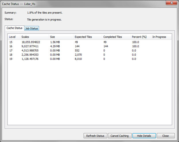
Figure 19. Cache Status window in ArcGIS Online, showing the number of tiles needed at each resolution (scale) level and the progress (in this case 1.8% complete) of the tiling operation.

17. While waiting for the tiles to be generated, you can login to ArcGIS online in a web browser, but stop after you have navigated to the My Content page (see instructions below).

7.6b Building an ArcGIS Online Map for use with the Collector App

After the three services (editable features, non-editable features, and Lidar hillshade) have been published to ArcGIS Online, they can be added to an ArcGIS Online map, then exported to the Collector app for offline use.

1. Open a web browser and navigate to the ArcGIS Online sign in page and enter your login credentials. https://www.arcgis.com/home/signin.html
   
   
2. At the top of the page, click the "My Content" tab on the top menu (see Fig. 20 below).

Figure 20.  The ArcGIS Online menu, showing the Content option.

3. If all has gone well with the service publishing from the previous steps, you should see your published layers as shown in Figure 21 below.  We will find it useful to collect photographs at points - these need to be "attached" to the points.  To do so we need to "Enable Attachments", which is done with a click for each feature class, shown in the red box in Figure 21a below.  To access the properties of a feature layer, click on its name to see the Layers as they appear in Figure 22 below. When completed these should read "Disable Attachments".

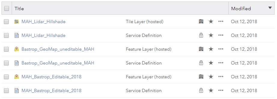
Figure 21. My Content window in ArcGIS Online, showing published layers.

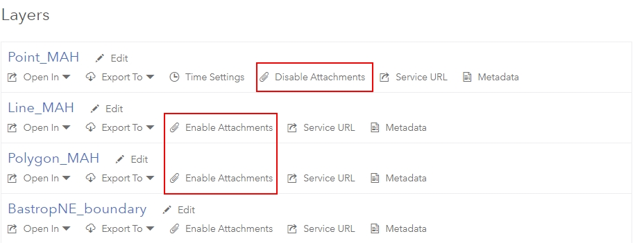
Figure 21a. Enabling Attachments in the editable Feature Layer.  In the view above, attachments are Enabled for the Point_MAH layer but not the others.

4. Your Lidar hillshade needs to be modified to permit offline use. Click the ellipsis (...) of Lidar hillshade Tile Layer, then click "View item details".
   
   
5. Click the "Settings" tab (Fig. 22), then navigate to the bottom of the page.

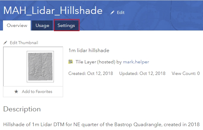
Figure 22. The Lidar Hillshade "View Item details" window in ArcGIS Online, showing the Settings tab.

6. Ensure the option for Offline Mode is checked (Fig. 23), then click "Save".

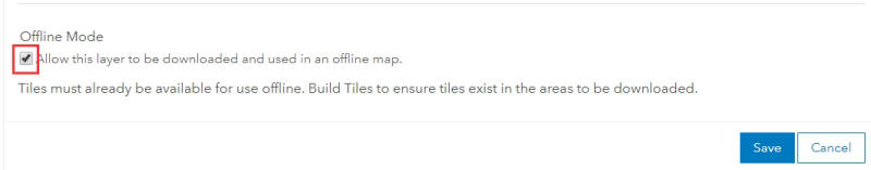
Figure 23. The enable Offline Mode option turned on will allow use of this Feature Layer without a WiFi connection.

7. Click the "My Content" tab at the top of the page.
   
   
8. On the ellipsis (...) for your Lidar hillshade Tile Layer, click the option to "Add to new map".
   
   
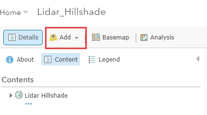
9. This should open a new map document with your hillshade displayed. Click "Add" at the top left portion of the screen (see figure below), then Search for Layers.  Set "In:" to "My Content" to see only your layers.
   
           
   
   
10. You should see all of the services you’ve published displayed. Click the "Add" button (the circled + icon) next to your editable features layer and your non-editable features layer.
    
    
11. Reorder the layers so that your editable layers (Points, Lines, and Polygons) are at the top of the table of contents.  Do this by click on "Details" and drag, using the icon visible when mousing-over on the left edge of each table of content item.
    
    
12. At the top of the screen, click Save> Save As.
    
    
13. Give the map a title that includes your initials, some tags, and a description.
    
    
14. After your map is saved, click Home> Content at the top left side of the screen.
    
    
15. You should see your newly saved map (a "Web Map") on your My Content page.
    
    
16. Your map should now be visible by the Collector app when you sign in to your ArcGIS Online account from the Collector App on a mobile device, either your phone and/or the iPad checked out to you.

 PART B  

Practice with the Collector App on an iPad Mini on campus

7B.1 Using Collector - some practice with the basics

1. Before our field trip, you need practice with Collector. An ArcGIS Online map for the Main Building area can be loaded on an iPad - ask Nicole for help if you can't figure it out on your own.  Take your instrument outside, open the Main Building project, and practice capturing lines, points and polygons.
   
   
2. Specifically, capture the features listed and labeled in the photo below.

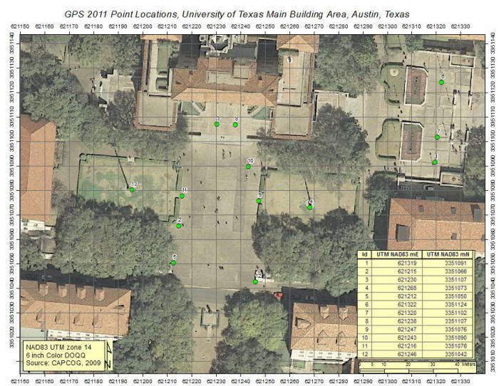
• Points: Points at the two flagpoles.
• L1, L2, L3: Polylines with at least 3 GPS vertices at the edges of sidewalks.
• P1, P2: Polygons outlining grass areas - capture a vertex at the 4 corners with GPS.

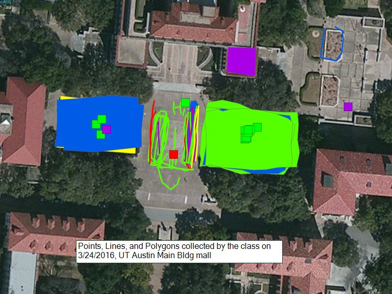
Below are some data captured last semester from all 15 iPads so you can get a feel for accuracy.  The squares are flag poles, lines are asphalt-paved areas in the sidewalks and polygons are the grassy areas enclosed by hedges that surround the flag poles.

You're done.

Mark Helper and Nathan Williams, Spring, Fall 2016