1.1 Purpose To become familiar with the following:
- The three modules of ESRI's1 ArcGIS Desktop
software
- Data display
- Basic cartography
And to provide the background necessary for future lab exercises.
1.2 Introduction and background
Computers
ArcGIS software is designed to run on a
variety of platforms (no Apple version, however). This semester our lab computers are running ArcGIS version
10.6.1 under Windows 10.
About the software
ArcGIS desktop is an integrated software package available at
three different licensing levels. The lowest and least expensive of
these is ArcView, once strictly a stand-alone program but now also a member of
the ArcGIS family. This is succeeded upward in price by ArcEditor
and then by ArcInfo. All contain the same three modules (see below) but
differ in the type and number of tools available for editing and
analysis. We will be using ArcInfo, considered the industry standard
by professional GIS users. In its current incarnation (version 8
and above), ArcInfo is a Windows-based GIS program - a significant departure from
versions 7.x and below, which used command-line driven, DOS- or UNIX-based
interfaces.
Importantly, ArcGIS at all three levels (ArcView, ArcEditor, ArcInfo) is structured around three key modules-
ArcCatalog, ArcToolbox, and ArcMap. These three modules represent
the three basic necessities of GIS - Data Management, Data Analysis ("geoprocessing"), and Data
Output/Mapping. This lab examines these three modules, exploring some of their
key functions.
ArcGIS Pro is a more recent
offering that has most of the same functionality as ArcGIS
desktop but designed to have the same look and feel as
ArcGIS Online (more on that later). We have
licenses and installations(?) of this most recent alternative to
ArcGIS desktop if you'd like to learn how to use it. I
have not yet adapted the lab exercises for it - a work in
progress that may be completed this semester.
Cartography
This lab also discusses some basic principles
of cartography. Those familiar with cartography will likely find this a review. The
intent is to provide basic guidelines and requirements for all maps that you will hand in. This is a very cursory
introduction; your skills in this area should improve throughout the
semester as you get feedback on your maps.
Among many good web sources, the
ESRI Mapping Center is a good place to start for information on
making great maps with ArcInfo. See particularly the
Maps
pages for nice examples and techniques to emulate.
Additional Resources
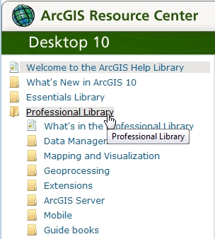
In
lieu of software manuals, all ArcGIS v.10.x documentation is now
distributed online at the
ArcGIS Help Library.
Most of what you will need is in the "Professional Library", accessible
in the menu on the left side of the web page (illustrated below).
This is your ultimate resource, and several specific links to it are
provided throughout the lab. Additional information on ArcGIS software can be found through the
ArcGIS web
site, and through the
ESRI
Virtual Campus web site, which offers several free modules on ArcGIS
and ArcGIS extensions.
Lab equipment
There is no required lab equipment for
this class, though it is recommended that you purchase a 2 Gb or larger flash drive to back up your lab
material and data. You are expected to store lab files and
data on a network drive, your so-called "r: drive". All students in
this and other courses share the same local hard drive space on the lab
computers, so there is the possibility that
work saved on a lab computer could be overwritten or deleted by others. To prevent this, we recommend copying
all of your lab work to your network storage space (r: drive) and/or a flash drive. Do not consider any work stored on a computer in this classroom
to be permanent. Use your
network storage space!
Note also that all classroom and lab computers
automatically reboot each evening at midnight. This
provides a "clean slate" for users each day but can result in
lost work if not saved before then.
Other information about the lab
Be sure you have
looked at your TA's Lab
Syllabus
and the other information on the
Labs page, such as
Software Tips,
Understanding
the Lab Format,
Layout Suggestions and the
Software Bugs page. Go no further,
READ OR EXPLORE THESE NOW.
1.3
Procedures
1.3.1 The Basics
Logging
in, mapping drives and creating folders Log in on a lab
computer. The class folder and your secure network storage
space should already be mapped to your profile. To find them,
go to My Computer and open the drive "files on austin
disk R:". There you should locate your UTEID, which is
your network storage space, and a folder called "geo-class",
which contains a folder with data for this course. This is an
essential first step - ask your TA for help if you can't do it. Creating
folders for your labs and lab data
Good computer file management in this class is essential.
Good computer file management in this class is essential.
Good computer file management in this class is essential.
There are two options for saving your data and lab work: a portable
flash ("thumb") drive or your network storage space on the Austin
disk. In later labs, flash drives will work better during lab
exercises than network storage (the software still has some bugs
when working with data across a network). Flash drives are great for
portability but can get lost, stolen or broken easily. With
many years of experience, your TA recommends working from a flash
drive and backing up all work to your Austin disk space at the end
of EACH work session. Whichever method you choose, begin today by creating a GIS class folder (give it a name less than
13 characters long without any spaces) and, within it, a
"Lab_1" folder. Do not put this folder or
any others within a "My Documents" folder. Follow this convention for all your
labs and life will be a little easier. Once you've created and
saved files for a lab, your life will also be much easier if you don't
move them from the location where they were first stored. This
can create broken links to data files, which can usually be fixed, but
it is easier and simpler to avoid this problem. We reiterate,
don't move files or folders around unless it is absolutely necessary. Note: DO NOT
PUT SPACES IN FILE OR FOLDER NAMES; use a "-" or a "_" instead. |
1.3.2 The Data
Copying
Data
Although it is possible to work directly from the Lab 1 data in the
class folder, DO NOT DO SO. Instead, copy the entire Lab 1 data folder,
called "Lab_1_data", to your Lab_1 folder
before beginning. There are a number of ways to do this - perhaps the
fastest is by dragging and dropping between two Windows Explorer
windows. Most importantly, when transferring these data, COPY THE
FOLDER, not the individual files within it. As will become
apparent later, certain types of files become unusable if copied piecemeal
without their hidden counterparts and without maintaining paths to other
files. Data for this lab are contained in two folders, Austin_Geo and
Texas_data, both of which reside in the Lab_1_data folder.
The Austin_Geo folder
contains:
- 7 shapefiles
(with extensions .shp)
- a layer file (extension .lyr)
- a map
document file (extension .mxd).
The Texas_data folder contains:
- state-wide data within a
geodatabase (extension .mdb),
- a folder that contains a state
transportation coverage
- a folder of geology layers and shapefiles
- a map document file that shows the geology of Texas
- a shapefile, "txtrct", the contents of which you
will determine.
Nearly all of these files are accompanied by a number of other
files with various 3 character extension, but having the same file name. The differences among these data types will be discussed in
upcoming class lectures and is briefly described below. After
copying the entire Lab_1_data folder (~94 Mb) to your Austin
disk space or flash drive, you will browse and
preview the various data using ArcCatalog. 1.3.3 ArcCatalog
Introduction to
ArcCatalog
ArcCatalog is the ArcGIS module used to
organize, browse, and manage your data and map files, as well as for
viewing and editing metadata (data about the data). In many ways, ArcCatalog is similar to
Windows Explorer. For instance, when you modify a file's location, or
create or delete a file, you do not need to save the changes -- it is done
automatically. Since it is easy to delete files this way, you should be
careful to delete only when you are sure that you will not need the file
any longer. Keep in mind that what you see in ArcCatalog is simply
an alternative view of your disk space(s), one designed specifically for
GIS data. Changes to data structure or files made with ArcCatalog
are the same as any changes you might make on your disk space(s) with
other software, like Windows Explorer. The
online resource for help with ArcCatalog can be found
here. Starting
ArcCatalog
Start ArcCatalog by navigating to All Programs -> ArcGIS ->
ArcCatalog.
The lay of the land, or,
What is in ArcCatalog?
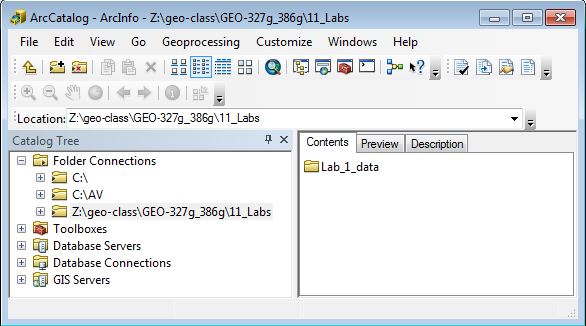
ArcCatalog is similar in structure to Windows
Explorer -- on the left-hand side is a view of a Catalog "tree" showing
how data are organized. On the right hand are options for
previewing the contents of the data shown in the Catalog tree. You will
notice that there are different icons for different data sources. Simple
folder icons link to and allow browsing of local disk space(s). Other
icons store links other data sources, some on the internet. As
seen above, these are Database
Connections, Toolboxes, GIS Servers, and Database Connections (not
discussed at this time).
At the top of Window are several menus and toolbars.
We will explore a number of these. Other
toolbars can be displayed (or turned off), by using the
"Customize">Toolbars menu option at the top of the window.
To determine what a particular tool does,
hold your cursor over the button for several seconds. A gray "tip" will
appear, telling the function associated with the tool. A more
informative description appears at the bottom of the ArcCatalog window.
For example, if you hold your cursor over the bent
upward pointing arrow (the first button directly under 'File'),
you will see the tip:"Up One Level"; the bottom of the window will,
at the same time, read 'Go to the next level up in the
catalog tree' (the ArcCatalog window must be the active window for this to
work).
Connecting to your
data
To access your data in ArcCatalog you have
several choices -- first, if there is already a connection to the disk
space
with your data, you can navigate down the catalog tree until you find your
data folder. If no such connection exists, you must create one.
You can make connections at any level of your disk space tree but it
often most useful to create a
direct connection to your data at the lowest level. A direct
connection will help avoid clutter because you can make a connection
straight to the folder holding your data, rather than having to navigate
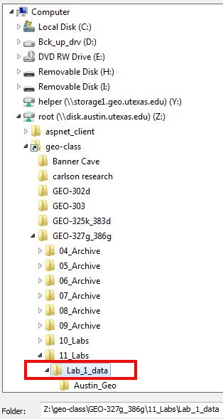
through other folders. An example of a direct connection can be seen in the graphic
in section 1.3.3.: note that the connection is to
"Z:\geo-class\GEO-327g_386g\2014_Fall_Lab_data" not simply to
"Z:\geo-class\GEO-327g_386g".
- Connect to your Lab_1 data, using the "Connect
to Folder" button
 ;
do not connect directly to the class folder. ;
do not connect directly to the class folder.
Navigate to the folder
containing your data for this lab- in the example to the right
(note: has not updated for Fall 2017 folders) Z:\...\2014_Fall_Lab_data\Lab_1_data. Select the folder (it
will highlight in blue), and then click "OK".
A direct
connection to your data folder will now appear in the Catalog tree. |
 |
Try this out again by connecting to a flash drive, and/or a folder
within the class folder.
What can I do in
ArcCatalog?
Earlier in the lab, it was mentioned that
ArcCatalog is used to "organize, browse, and manage your data and
map files, as well as for viewing and editing metadata." We'll
explore it a bit more: For organizing data, ArcCatalog is quite easy
to use. However, if you delete, move, or otherwise alter the data
using ArcCatalog, it is permanent (i.e., if you delete something from
your GIS folder, it is
GONE - you can not retrieve it). Data organizing in ArcCatalog
is very similar to that in Windows Explorer - you can drag and drop
coverages, shapefiles, or geodatabases into new workspaces, or you can use
the Windows shortcut keys (Ctrl-X and Ctrl-V).
Try this out by copying and pasting your lab
data into a new folder. (Delete the old folder when done.)
Browsing through your data is simple using
ArcCatalog - the Catalog tree displays, in a hierarchical fashion, all of
the items in the Catalog - much like how data browsing is done with Windows Explorer. A folder that contains files
will have a box with a plus or minus sign to the left of the file name.
This indicates whether or not the folder has been expanded.
Take a moment to explore the data in
the Catalog tree - use the arrow buttons on your keyboard or the mouse to navigate. While navigating, pay attention to the
changes that take place on the right hand side of the ArcCatalog
window.
The right hand side of the Catalog allows you
to examine the data further. For instance,
in the "Texas_data" folder, click the "USGS_TX_boundaries_GRS80.mdb" geodatabase. If you then click on the "Contents" tab on the right hand
side of the window (shown above), a list of the feature datasets and
feature classes in the geodatabase are displayed as icons (c.f. the icons in the
table above). You can also see these if you click on the
"plus" sign
to the left of the USGS_TX_boudaries icon on the left hand side, so
it's not very interesting to see these on the right.
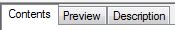
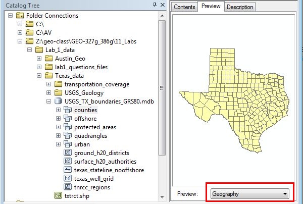
For something a bit more interesting, click on the "Preview" tab to see a preview of the data or the data attribute table. To change
from geography view to table view (or vice versa), use the "Preview:" drop-down menu at the bottom of the Window,
outlined in red below.
The screen capture below shows a Preview of the "counties" feature
dataset.
Question 2 When previewing data, a
previously grayed-out toolbar at the top of the window becomes
active. Why? What do the tools do? Are
they always active when previewing data?
|
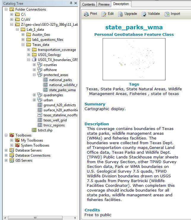
Click on the "Description" tab and browse to "protected_areas">"state_parks".
The right window, as seen below, shows "Metadata"
for this dataset, including a thumbnail image,
Summary, Description,
Credits, Access and Use Limitations. The metadata can be edited
(or created) using the "Edit" tool at the top of the
Description tabs. If the metadata must meet a certain standard
(e.g. such standards exist for Federal datasets) than it can be
"Validated" with the "Validate" tool. It can similarly be
"Imported" from another data source.
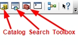
| Finding data and tools - The Search window
New in ArcGIS version 10 is a robust search capability. If set
up and used properly, it allows quick access to data and tools that
might otherwise be very hard to find. Search is accessed
through a search window, available in both ArcCatalog and ArcMap. We
will try it first in ArcCatalog.
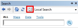
Click the search window icon
 near the top of the ArcCatalog window. This brings up a window
that is docked on the right side of the ArcCatalog window. It
can be undocked by clicking the pin in the blue bar at the top of
the window, then dragging the window by the blue bar to a new location. It can
be collapsed and hidden while docked by clicking the "pin" icon in the
blue bar, and it can be re-docked by dragging the window back into
ArcCatalog.
near the top of the ArcCatalog window. This brings up a window
that is docked on the right side of the ArcCatalog window. It
can be undocked by clicking the pin in the blue bar at the top of
the window, then dragging the window by the blue bar to a new location. It can
be collapsed and hidden while docked by clicking the "pin" icon in the
blue bar, and it can be re-docked by dragging the window back into
ArcCatalog.
**A
data search will only be successful if the data storage area/folder/internet
resource/etc. is first indexed.** You will want search
capability for your network drive, so it needs to be indexed.
With appropriate modification, duplicating the steps below will
allow searching of other locations as well.
- Open the "Index/Search Options" (in red below);
- Use the "Add..." button to browse to
your network disk space and then click "Select".
- Set the Indexing Options so that new
items on your disk space are Indexed every 60 minutes and are
Re-Indexed from scratch every 6 days, starting at 1 AM.
- Click Apply and Indexing will begin.
Click OK and indexing continues while you work on other things.
Once indexing is complete, the software searches by file
names, words in metadata ("Tags") and key words in the software (for software
tools). This will be an extremely valuable tool as the
semester progresses; learn to use it!
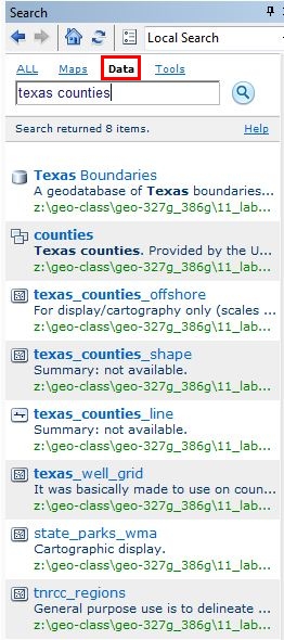
After waiting a few minutes to build an Index,
give it a try: We will search for Data, so click the
underlined "Data" (shown with red box below) before typing in "Texas counties". The result
should look something like that below. Mousing over a result
provides a preview of the data; clicking the green link will take
you to it in the ArcCatalog tree.
Question 3:
Within the USGS_TX_boundaries geodatabase,
the "counties">"texas_counties_shape" feature dataset's
attribute table contains fields for AREA and PERIMETER. The
values are in square meters and meters, respectively. Use
Table Preview to find areas and perimeters
of the counties in the table below. Convert your answers into
square kilometer and km. Hint: right-clicking on a column heading
in the table allows you to sort/reorder the table rows.
| County |
Area (square km) |
Perimeter (km) |
| Travis |
|
|
| Llano |
|
|
| Williamson |
|
| |
Question 4:
Examine the metadata for the geo.shp file in the Austin_Geo
folder. Where did these data come from and upon what are they
based? |
Managing
your data
Managing your data is
also done in ArcCatalog. You can examine and/or modify the
properties of your data simply by right-clicking on the file icon in the Catalog tree and selecting
"Properties. Do this for
the faults.shp shapefile in the Austin_Geo folder.
Different file types have different Properties windows. For shapefiles, like that you are now
examining, you should see a window like the one below. The tabs
contain various types of properties:
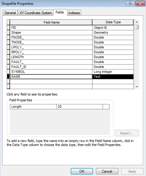 |
General
-- for shapefiles, a name and alias (a more complete or different name) is listed. The same tab for a coverage (see
highways_dd in the Texas_data folder) or geodatabase contains other
information, discussed in later labs.
Fields --
lists the attribute table field (column) names and their types and
properties. Clicking on the "Name" Field Name brings up a
description of the Field Properties, (a Text field with a length of 20
characters, as shown in the image on the
left. Field Properties will be discussed later.
Indexes -- contains a list of
fields for which indexes can be created, speeding search and query
operations.
XY Coordinate System -- all spatial datasets (e.g.
points, lines, areas) are stored as tables of x and y (also
sometimes z) coordinates. Coordinates are referenced to a set
of X and Y axes (a coordinate system), and to a particular model of
the shape of the earth (a datum). This tabs show the datum and
coordinate system used by the dataset. |
Explore the Properties for the
highway_dd
coverage and the geo.shp file.
Question 5:
What is the "Spatial Reference" (i.e. XY Coordinate System) for
highway_dd and geo.shp? |
1.3.4 ArcToolbox
Introduction to ArcToolbox
ArcToolbox is the ArcGIS module for
geoprocessing. ArcToolbox also provides
an option to write scripts and create customized data
processing/ analysis/conversion tools.
Starting
ArcToolbox
To start ArcToolbox, click the toolbox
 icon in the ArcCatalog
toolbar. icon in the ArcCatalog
toolbar. |
What is in ArcToolbox?
As you can
see when looking at ArcToolbox, it provides tools for "geoprocessing" - Data
Management, Analysis, and Conversion. Let's
explore the organization of ArcToolbox a bit more:
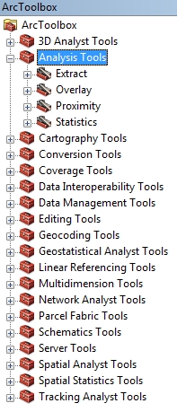 |
ArcToolbox is organized in a fashion
similar to the catalog tree in ArcCatalog. By clicking
on the + next to a toolbox heading (Data Management Tools,
Analysis Tools, etc.) you can open that toolbox to view its tools or
other toolboxes.
In the figure to the left, the "Analysis Tools" toolbox is open to
show the "Extract", "Overlay", "Proximity" and "Statistics"
toolboxes.
To use a tool, double-click on the
 icon for the tool.
Doing so brings up a "wizard" window that provides brief
explanations of the fields where you will enter information. It also
contains a "Help" button that takes you to a full explanation of the
tool. We will have many occasions to use tools within some of
the toolboxes, beginning next week with Data Management Tools for
Projection and Transformation. icon for the tool.
Doing so brings up a "wizard" window that provides brief
explanations of the fields where you will enter information. It also
contains a "Help" button that takes you to a full explanation of the
tool. We will have many occasions to use tools within some of
the toolboxes, beginning next week with Data Management Tools for
Projection and Transformation.
As stated above, one of the principle differences among the three
licensing levels of ArcGIS (ArcView, ArcEditor, ArcInfo) is the type
and number of tools available in ArcToolbox. Our ArcInfo license includes every tool available.
With so many tools available, searching for the right tool by
simply looking in each tool box becomes onerous. A better
approach is to instead use "Search" window
described above, but
with the "Tools" option instead of the "Data" option.
|
|
Take a few minutes to explore the
toolbox and the "geoprocessing" options provided.
Few will make sense to you now, but you will at least get a feel for
their vast numbers. |
Question 6:
Use the Search window to find a list of
"projection" tools (use "projection" as the keyword).
a.) What toolbox contains the "Define Projection" tool?
Open the Define Projection tool wizard window.
b.) What does the Define Projection tool do?
|
1.3.5 ArcMap
Introduction to ArcMap
ArcMap is the ArcGIS module for creating, viewing, querying, editing,
composing, and publishing maps. We've saved the best for last...
Starting ArcMap
Similar to ArcCatalog, ArcMap can be opened
via the Windows Start menu (Start -> All Programs -> ArcGIS -> ArcMap) or
from ArcCatalog (click on the  ArcMap
icon). In addition, you can open ArcMap by double clicking on any map
document file ArcMap
icon). In addition, you can open ArcMap by double clicking on any map
document file  visible in the catalog tree of ArcCatalog
or Windows Explorer. visible in the catalog tree of ArcCatalog
or Windows Explorer.
When you first start ArcMap, you get the "Getting Started" window - this window provides the options to: 1)
Create a new empty map; 2)Open an existing
map; or 3) Create a new map using a map template. This semester we
will most often use options 1 and 2.

The other important feature of this opening window, as shown above in
the red box, is the "Default geodatabase for this map:". By
default, this is set to a location on the local computer, usually your
My Documents\ArcGIS folder (this is automatically created when you open
the software), where you may or may not be able to find your work.
Read the "What is this?" hyperlink, highlighted by the red
arrows above, for a complete explanation of this
feature. In later labs, when we begin to work with Geodatabases,
you will change this default location.
Using the "Browse for more..." option, open the prepared map document Austin_Geo_G-Y.mxd
in the Austin_Geo folder. You can open this from the Welcome window, or when ArcMap
is open, click on File -> Open..., and navigate to the location of the map file.
From within ArcMap,
Open ArcCatalog and Search with the buttons at
the top of the window (shown below). Dock them on the right side of the
ArcMap window, and reduce them to tabs.
What is in ArcMap?
Before going any further,
careful read and study
A Quick Tour of ArcMap,
an excellent summary of the basic features of ArcMap. As you do so,
refer to your the map document open in ArcMap.
Some important highlights:
- The top portion of the ArcMap window
contains the menu and toolbars. You can change which toolbars are
displayed by right-clicking on the top portion of the window (the
gray part) and selecting which toolbars you need or don't need.
They can be docked or undocked by dragging the left end of the toolbar.
- The left portion of ArcMap is the Table of Contents (TOC). It shows a
layers icon
 that
denotes a Data Frame. As the name suggests, a Data Frame is a
conceptual rectangle that encloses all of the data that are needed for a
particular analysis, for display, or for part or all of a printed map.
Most of these data will occupy layers, but others may simply be database
tables. Like the files we examined in ArcCatalog, Data Frames have
properties that can be explored by a right-click on the Data Frame name,
or by asking for "Data Frames Properties..." beneath the View menu at the
top of the window. Map documents can have more than one Data Frame,
but only one at a time can be displayed or analyzed. The Austin_Geo map
document has a single Data Frame, titled "Garner&Young NAD83"
(F.Y.I. Garner and Young are the authors of the original paper map and
NAD83 is the datum for the coordinate system of all the map data). that
denotes a Data Frame. As the name suggests, a Data Frame is a
conceptual rectangle that encloses all of the data that are needed for a
particular analysis, for display, or for part or all of a printed map.
Most of these data will occupy layers, but others may simply be database
tables. Like the files we examined in ArcCatalog, Data Frames have
properties that can be explored by a right-click on the Data Frame name,
or by asking for "Data Frames Properties..." beneath the View menu at the
top of the window. Map documents can have more than one Data Frame,
but only one at a time can be displayed or analyzed. The Austin_Geo map
document has a single Data Frame, titled "Garner&Young NAD83"
(F.Y.I. Garner and Young are the authors of the original paper map and
NAD83 is the datum for the coordinate system of all the map data).
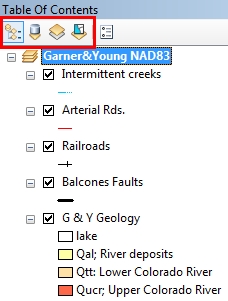
Below the Data Frame name is
an expandable tree of five layers, which are presently unexpanded but
turned on for display. There are several ways
to view the TOC - presently they are displayed by Drawing Order; the
topmost layers are drawn on top of the bottom-most layers.
The layers can be also be viewed by source, visibilty and
selection (to be explained later). You can toggle between
the views by selecting the appropriate icon at the top of the Table of
Contents window, shown below in the red box.
|
|
- With the "Drawing Order" view, the TOC shows the layer name, whether
or not the layer is turned on (a check in the box next to the name indicates such), and symbology for the layer (to see this, click
on the + to the left of the name to expand the tree; the expanded tree
is shown above).
Alternatively, the "Source" view shows the location (or "source") of the data. We generally work
with the TOC in Drawing Order rather than Source mode, but Source mode is useful
when trying to keep track of where data are stored, and it is needed to
see stand-alone tables. A third choice, "List by Selection", provides an
important way to choose which layers are available for "selection" by
tools we will explore later.
- The central portion of the ArcMap window provides a view
of the layers that are turned on in the TOC, in other words, the map! Three very important small buttons
 in the lower
left corner of the map viewing window provide a means of viewing data in
"Data View" , "Layout View" or a way to refresh (redraw) the view. The
left icon brings the 'data view', the middle icon brings the 'layout view' and the circular arrows
redraw the map window. These buttons are easily lost among
everything else, but they are extremely handy. The same functions are
available under the "View" menu at the top of the ArcMap window. in the lower
left corner of the map viewing window provide a means of viewing data in
"Data View" , "Layout View" or a way to refresh (redraw) the view. The
left icon brings the 'data view', the middle icon brings the 'layout view' and the circular arrows
redraw the map window. These buttons are easily lost among
everything else, but they are extremely handy. The same functions are
available under the "View" menu at the top of the ArcMap window.
- While in either Data View or Layout View, you can zoom in, out,
pan, identify, select, measure etc. map data in the map viewing window by using the
tools of the "Tools" toolbar:

Tools Toolbar - I like to dock this on the left side of the ArcMap
window.
A
table in the Help
files explains the function of each of the tools in this toolbar.
Zoom in and out and otherwise
explore the data using the above tools. Use the ArcMap Help
menu at the top of the ArcMap window for a full explanation of
the Select Features and Identify Tools, two of the most useful but least intuitive tools on this toolbar. The globe and blue
arrow tools are also invaluable - they will return you to either a
view of the entire data set or to the previous viewing extent.
Get used to using these tools-they are far more effective and
efficient than the magnifying glasses for many operations. (Conversely, I find the
fixed zoom in and out tools of little use.)
Before going further, read and study "Using
data frames".
Notice that as you
zoom in and out, line thicknesses, labels, etc. change size.
When zoomed way out, some things become nearly invisible. What controls
this, and will you have to redo all the symbols every time you want to
look at or print a map at a different scale? No. The
answer is contained in a map "reference scale". All symbols,
labels, etc. are drawn to their proper relative sizes only at an
assigned "reference scale" for the map. Zooming out and in takes
you away from the reference scale and symbols appear either too small
or too large. To restore the symbols to their proper relative
size, either 1) return the display to the reference scale, or
2) reset the reference scale to match the scale of the display.
Both of these extremely important functions are accessible by a
right-click on the Data Frame name (i.e. Garner&Young NAD83) in the
TOC, then selecting the "Reference Scale" option and either "Zoom To
Reference Scale" or "Set Reference Scale", as seen below.
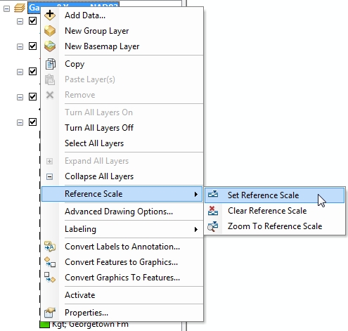
I set the reference scale for this map at 1:24,000.
Zoom to some other scale, either way out or in, and reset the
reference scale ("Set Reference Scale") by the technique described
above. Notice the effect. Get used to performing this very
important function. |
After exploring the map in Data View, go to the
Layout View - you can do this by either clicking on the sheet of paper
icon at the bottom of the view window
 , or by selecting View->Layout
View from the menu at the top of the ArcMap window. , or by selecting View->Layout
View from the menu at the top of the ArcMap window.
Before going any further, carefully ready and
study "A
quick tour of page layouts".
Layout View gives a What-You-See-Is-What-You-Get preview of a printed
page. A page, its margins, a set of rulers and the Data Frame
layers that are turned on are shown. The size of the page that is
displayed, landscape vs. portrait mode, etc. are set under the File
->Page Setup menu. We will explore Page Setup properties during a
later lab - for this lab leave them alone.
The actual Data Frame is visible by clicking on
the map, which brings up a dashed box with blue vertices that can be used
to enlarge or reduce the size of the Data Frame. Try it and see.
A somewhat confusing aspect of Layout View
is a new set of tools on a Layout Toolbar, shown below. While
these tools superficially appear to perform nearly identical functions to those of the
Tools Toolbar, they do not.
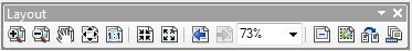
The Layout toolbar. I keep this docked on the right side of the
ArcMap window.
The key thing to remember about these
tools is that they operate on the page itself, not the Data Frame.
For example, zooming with the magnifier tool of the Tools toolbar will
change the map scale (displayed near the top of the ArcMap Window),
whereas zooming with the magnifier on the Layout toolbar simply gives you
a closer look at the page; the scale of the data frame remains the same.
Try it and see.
First, get the entire map visible in the Data Frame of the Layout
View. One way to do this is by typing in an appropriate scale in
the scale window
 near the
top of the ArcMap window. 1:200,000 works nicely for these data. near the
top of the ArcMap window. 1:200,000 works nicely for these data.
- Now, using the Magnifier and blue Back Arrow key of the
Tools toolbar, alternately zoom in
and return to different scales, noting the change in the area of
the map displayed on the page and R.F. scale in the scale window.
- Return the map to a scale of 1:200,000.
- Next, do the same with
the two similar tools on the Layout toolbar. Note the difference
- the scale does not change in the scale window, meaning that you are
simply seeing a magnified view of the page, not changing the scale or
region of the map that will eventually be printed.
Two particularly useful layout tools are the Zoom to 100%
 and Zoom
Whole Page and Zoom
Whole Page
 tools. tools.
|
Question 7
Explain what the "Zoom to 100%" and "Zoom Whole Page" tools do. |
While in Layout View, to insert a title, legend,
neat line, etc. on your map, use the "Insert" menu, shown
below, and select the
object that you would like to add.
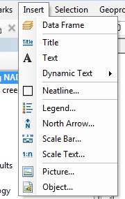
Experiment with adding information to your map -
from the "Insert" menu try adding a title,
legend, scale bar, north arrow, and your name. The drawing tools at
the bottom of the window can also be used to insert text, draw and
fill boxes, polygons, etc, and to format text. You may want to use this
map file later in the lab, so save your changes.
Do so with
a new file name in your Lab_1
folder.
|
Adding data / Creating
your own map
Now that you have spent time with a pre-made map file, it's time to
make your own.
In ArcMap you cannot have two
map document (.mxd) files open at the same time, so to open a new map file we
either need to open a new ArcMap window or close the existing map file. In
this instance, since we will not need the Austin_Geo_G-Y map document for this
portion of the lab, click on File -> New (or you can use the shortcut
key "Ctrl-n", or click on the new map file button on the menu bar), and select
"Blank document."
Before proceeding, read
Adding layers to a map. Highlights:
Three ways to add data to a map:
1. Use the "Add data" button on
the ArcMap toolbar

2. Navigate to File -> Add data
3. The quickest method: Drag and drop data from ArcCatalog.
With ArcCatalog open within ArcMap, left-click
and hold onto
the data file in the ArcCatalog tree that you want to add to your map -
hold the mouse button down, do not release the button yet. Drag the
data straight from ArcCatalog to a Data or Layout View window in ArcMap,
or into the TOC. Release the
mouse button and the data will load into ArcMap.
Try each of these methods to add the
texas_counties_shape feature class (in the geodatabase under the
"counties" feature dataset), and the clip_TX_Faults and
txtrct shapefile to your new map file. Answer OK to any warning
messages that may appear.
|
|
Question 8
What data are contained in the txtrct shapefile? Where did they
come from? |
| |
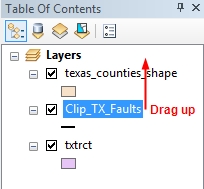 |
Order of data layers:
Depending on the order in which you added the data, your counties may
be "on top" of your faults (in which case the latter would not be visible on the map). You can change this by
clicking and dragging data layers "on top" of other data layers, just
as you might do in Photoshop or Illustrator.
This example shows moving the
clip_TX_Faults on top of the
texas_counties_shape layer. |
Learn more about Table of Contents functions in this
valuable link:
Using the table of contents. Data properties: In ArcMap,
to view the Properties of a data layer, double click on the data layer's
name. This will take you to the very important Layer Properties window. Note: The ArcMap
Layer Properties window will provide different information than
was found in the ArcCatalog Properties window.
You can also do this by right-clicking on the
data layer and selecting the Properties option. From the properties
window you can view and modify numerous properties of a dataset -
including the layer's transparency, labeling options, symbology, and
source. This lab will only cover a few of the options (display, symbology),
but you will want to take a few moments to familiarize yourself with
some of the other tabs in the properties window. The Layer
Properties windows is perhaps the single most important tool for
understanding, symbolizing and displaying data layers. Get used to
viewing Layer Properties by routinely right-clicking on the layer name
in the TOC.
Symbology: Under the symbology
tab are the options for how data are symbolized. From here you can decide to
display the data as Features (single symbol), Categories (unique values,
unique values many fields, or match to symbols in a field), Quantities
(graduated colors, graduated symbols, proportional symbols), or Multiple
attributes (quantity by category). You can also decide what color(s)
and symbol(s) to use to represent the data.
To see a short overview of
symbols and styles read
Using symbols and styles.
For example, the fault
layer actually contains dashed faults, dotted faults,
and a few hidden contacts. We would like them to
display differently ("uniquely"). To do so,
- double-click on Clip_TX-Faults in the TOC
to open the Properties window, then click the
Symbology tab. As the default, Clip_TX_Faults
is drawn as
a single symbol.
- Since we want to show all of the different types of
"faults",
we will use Categories -> Unique values. Before we can do
so we need to know what information there is about fault
types stored with this file. This information is
in the files "Attribute Table".
- A quick look at the Faults Attribute Table (right click, "Open Attribute
Table"; this could also be done by previewing the table in ArcCatalog)
shows that the fault line types are contained in a field called LTYPE
and described in the field LONG_DESC. Although we could use
either, we want to symbolize using the LONG_DESC field because it
contains a written description of the line types that will show up in
the symbol legend - it will save us some typing.
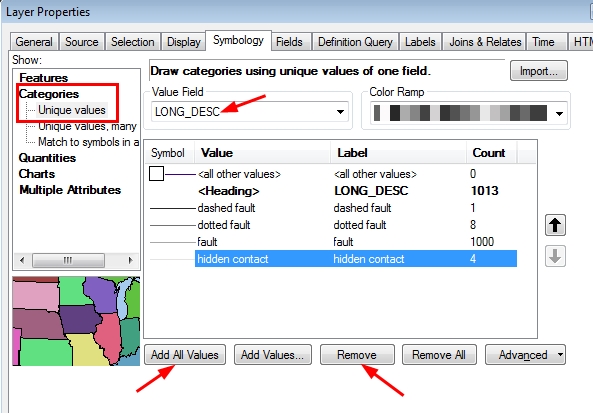
- So... after
going back to the "Symbology" tab in the Layer Properties window for the
Faults layer, from the "Show" window select
Categories, then "Unique Value", then in the
"Value Field" choose LONG_DESC from the
drop-down list (see the picture below). To see each of the
unique values in the LONG_DESC field, click the "Add All Values"
button.
- Hidden contacts aren't faults, so we'd like to remove them from the
map. To do so, click on "hidden contacts" in the "Value" column of
the Symbology widow and then click the "Remove" button. To add them back
in we can use the "Add Values.." button or "Add All Values" button. We can
selectively add any or all of the line types with the "Add values"
button. To change the symbology of other data layers (even of other
types of data -- e.g. coverages or geodatabase) the process is generally the
same.
|
Question 9:
What other information is provided by the symbology
tab for the LONG_DESC field? From this window, in
what ways can we change data representation?
|
Symbology and data appearance (Cont.)
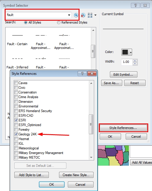
- To change the fault line
types and colors, double click on the line next to the name
and select an appropriate line symbol from the Symbol Selector.
Standard fault symbols are available in a pallet that can be loaded
into the Symbol Selector by clicking the "Style References..." button and
selecting "Geology 24K". Change all fault values to appropriate symbols
by first using the search in the symbol selection window to search
for "fault".
See the diagram below for hints.
- Colors and line width can be adjusted as well. Uncheck the <all other
values> symbol in the symbol column of the Symbology tab. When
everything is to
your liking, click OK and examine the result, both in the TOC and the map
view window.
|
Display
An important feature of Layer Properties is a
Display tab that allows the option to set transparency. This allows
for a layer to be seen through another layer. For lab this week,
this is not a critical feature, but we will find it very useful in coming
labs. To explore this, we'll make the texas_counties_shape
layer partly transparent.
Open the properties window for this
layer and select the Display tab. Under " %
Transparent" enter 75 and click OK. This noticeably dims the
counties and their boundaries, making the faults more visible for display.
We might also be able to visually determine the extent to which Texas
census tracts coincide with Texas counties this way, by making either the
census data or county data dim enough to see through. Try it and
see.
Saving and Reopening Map Documents
Since it is likely that you will open data from both your
network drive and from copies on your local drive, it is helpful to use a
relative path to a map's data layers. This will be handy if you copy your lab
data folder to a local drive to work, or if you move it from one drive to
another. If you do not store your data sources as relative path names, you
will run into the problem of ArcMap looking for the data on the last drive
which you used (e.g., if you create a map document with your data located in
Y:\Lab_1\; and you then copy the entire folder to another drive, when you
open the map file from the new folder, it will still look for the data in
Y:\lab1). A relative path name tells ArcMap to look for the data in the
same location relative to the map document file- e.g., in the same data
folder, or wherever it is in relation to the map document file.
To set your map document to use relative path names, click
on File>Map Document Properties, then check "Pathnames: Store relative
path names to datasources". Click OK. Note: You will probably want to do this with
ALL map files that you create in this course. Do this routinely when
beginning a new map document.
Occasionally, even if you set the map file to use relative
path names you will still have problems with broken sources. These will be
indicated by a red ! next to the layer's name,
e.g.
To fix this problem, click on the red exclamation point
and reset the source to the appropriate location by browsing to the data's
location. ArcMap is somewhat smart - if you fix one broken source
location, others will be fixed automatically if they too are at the same
location.
Other Slick Tricks in ArcMap
- When you have zoomed to an area of
interest, you can set a spatial bookmark. A spatial bookmark will
allow you to zoom to exactly the same area whenever you want. To set the
bookmark, select View -> Bookmarks -> Create. To return to a
bookmarked view, select the bookmark from the list you create
under View->Bookmarks.
- "Overview" and "Magnifier"
window are available under the Window menu. Try them;
they're very cool and self explanatory.
(VERY) Basic
principles of cartography(courtesy of David Jones and M. Helper)
-see also
Layout Guidelines and the "Best_practices_Maps"
folder in the class folder.
- Data in maps:
- The data should take up a majority
of the area; avoid excess white space.
- Inclusion of unnecessary data should be
avoided; simpler is better.
- Bright, flashy colors such as red should not be used
unless you specifically need to do so.
- Titles:
- Should usually be in upper case.
- Should not be sentences, but should
be simple and to the point. For maps, a title should contain
the subject of the map (e.g. Geologic Map of ....) AND the
location (...Travis County, Texas)
- Should not be the focal point of your map.
- Should almost always be black or dark
text.
- Should be placed in a
location on the map so as to not obstruct any other portion of the
map.
- Scale bars:
- NEVER have a scale bar that extends all the
way across a page. Scale bars should not be the focal point of the
map, they are for reference only.
- Scale bars should use appropriate measurement systems.
Example: km for Travis County, meters for the UT campus.
- Use intervals that
make sense. Units of 2,5,10, 20 are common. For example, do
not use intervals of 23.4, or even 23. Note that the ESRI
default scale bar properties allows the interval values to
change when the scale bar is lengthened or shortened.
You will always want to change this default so that the
interval is fixed to avoid awkward interval values.
The default scale bars are also (IMHO) too thick and use
characters that are too large.
- Borders:
- Maps need borders, they should usually be
black.
- Borders are known as
"neat lines."
- Neat lines
should not detract from the focus of the map, i.e. overly thick or
dark.
- North Arrows:
- Should be
unobtrusive.
- Are unnecessary and misleading on maps of
large areas at small scales, i.e. where lines of longitude would
show noticeable curvature.
- The default size of the ESRI default north arrows are
universally too large - scale them down on your maps.
Likewise, the original intent of map north arrows was not
decorative; they were the practical means of precisely
orienting a map! Some of us still use them that way...
- Legends:
- Legends should be unobtrusive
- Legends should only show features that are not labeled
on the map or aren't obvious from universally recognized
symbols.
-
Text on Map:
- Text should NEVER cross other text or other
features of the SAME color.
- Labels for natural features such as streams, lakes etc. should be
in italics.
- Text
should be legible! Save or print your final product at the
reference scale of the map so that all symbols and text are properly
scaled.
-
Name on Map:
- Unless the map is being published, names should
be kept outside of the neat line. For this class your name can go
above the neat line
in the upper right corner.
- White Space:
- Do not waste space. Try to find the
balance between too much white space, and cluttered data.
- Color:
- Selection of colors for map
data can make all the difference... A
particularly good source of color advice for
cartography is
Cynthia
Brewer's ColorBrewer 2.0 site, which
includes suggestions for colorblind safe
palettes.
|
Your map for Lab 1:
Using no more than 4 of the
data files in the Lab_1_data folder, construct a color map.
Follow the above listed principles of cartography and those in the
layout guidelines. In addition to the above, the map should have a title, scale bar,
explanation, your name and the date completed.
|
1.4 Conclusion
In this lab, the basic functions of ArcGIS's
ArcCatalog, ArcToolbox, and ArcMap were explored. You may not
yet feel comfortable navigating the software, the Geology Building network, and the lab computers,
but you will. True mastery (if there is such a thing) comes only
with prolonged practice. Keep at it - spend as much time as possible
working with the software and with these computers.
As with any new software, these basics do not
come close to being comprehensive - to really grasp the software,
you will need to spend quite a bit of time just exploring, trying out
different functions, seeing what works (and what doesn't), and just
clicking on buttons, menus, bits of data, and especially the help
files. Don't be afraid to explore. You can always Exit and
start over.
|
1.5 To Turn In
-
The question sheet (available in the Lab_1_data class folder), with
typed answers
- Your map
|
1 From an ESRI
publication: "Founded in 1969, ESRI ( Environmental Systems Research
Institute) is the leading developer of GIS software with more than 300,000
clients worldwide. ESRI software is used in all 200 of the largest cities
in the United States and in more than 60 percent of counties and
municipalities nationwide. Headquartered in California, ESRI has regional
offices throughout the United States, international distributors in more
than 90 countries, and more than 2,000 business partners. ESRI’s goal is
to develop comprehensive tools that enable users to efficiently manage,
use, and serve geographic information to make a difference in the world
around them. ESRI also provides consulting, implementation, and technical
support services. ESRI can be found on the Web at
www.esri.com."
Back
|
|